Modified Tortuosity Index: Tolerance Sensitivity

Summary

When determining the Modified Tortuosity Index (MTI) for as drilled well trajectories (versus planned trajectories), the calculated values can be sensitive to the chosen tolerance values used to check for normal vector (and Dog Leg Severity) continuity. This post investigates these sensitivities, recommends standard tolerance values and describes a method of assessing as drilled tortuosity versus planned tortuosity and proposes a Key Performance Indicator (KPI) for assessing the quality of a drilled well trajectory.

Disclaimer

The following method is experimental and has yet to be thoroughly tested - the work presented is that of an enthusiastic amateur, with no professional or otherwise affiliations. As such, please use with caution and do your own research and testing - the only request is that, in the spirit of open source you report back your own findings either via the comments below or via the welleng repository. The license is permissive - the only requirement is that you reference the source if you use the method or code.

Background

A previous post describes a methodology for determining the Modified Tortuosity Index (MTI). This method splits a well trajectory into curve turn or hold sections by assessing the continuity of successive survey station normal vectors. A tolerance is utilized when making this continuity check and in the post a value of 1.0 was recommended, which works well for planned surveys but is perhaps too coarse for as drilled surveys.

Import Some Well Data

We’ll start by importing an as drilled well trajectory survey. For this, we’ll utilize the NLOG Dutch Oil and Gas portal where surveys for all the wells drilling in the Netherlands can be downloaded here.

To make things interesting, we’ll select the longest well in the database as likely this will have a fair amount of tortuosity. That happens to be the well with NITG_NR reference BK050073, which for convenience has been extracted from the data and is available here in json format.

Here’s the code to import the json file and assign to the variable data:

import json

filename = 'assets/data/2022_06_11_BK050073.json'  # change to point to your file

with open(filename) as json_file:
    data = json.load(json_file)

Now we’ll create a Survey instance and do some quick QAQC:

import welleng as we

survey = we.survey.Survey(
    md=data['data']['AH_DEPTH'],
    inc=data['data']['DEV_ANGLE'],
    azi=data['data']['AZIMUTH']
)

A quick visual QAQC can be done with the following console command:

>>> survey.figure().show()

This should pop up the following chart in a web browser (a decent Extended Reach Drilling (ERD) well):

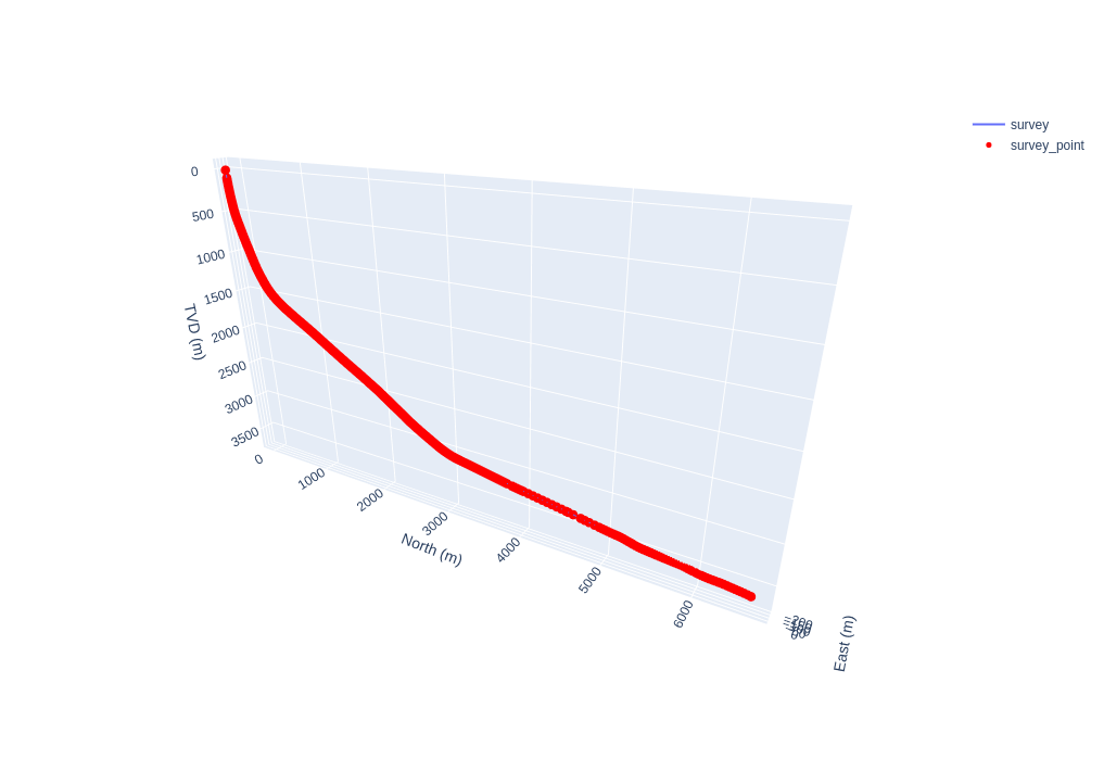As drilled trajectory NITG_NR: BK050073 from NLOG.

Tolerance Sensitivity

Now we have a well, lets see the impact on the MTI result of the tolerance parameter. We’re going to be trying out a few different values for rtol and we will want to see the results versus the as-drilled survey, so we’ll write some functions todo this for us:

from copy import deepcopy
import json
import numpy as np
import plotly.graph_objects as go
import welleng as we


def get_survey_mti(survey, rtol=1.0, **kwargs):
    mti = survey.modified_tortuosity_index(rtol, data=True)
    starts = np.hstack((deepcopy(mti['starts']), len(survey.md) - 1))

    # build up a trajectory from the mti control points
    connectors = []
    for i, (u, l) in enumerate(zip(starts[1:], starts[:-1])):
        if i == 0:
            connectors.append(
                we.connector.Connector(
                    md1=survey.md[l],
                    pos1=survey.pos_nev[l],
                    vec1=survey.vec_nev[l],
                    pos2=survey.pos_nev[u],
                    dls_design=1e-3
                )
            )
        else:
            connectors.append(
                we.connector.Connector(
                    node1=connectors[-1].node_end,
                    pos2=survey.pos_nev[u],
                    dls_design=1e-3
                )
            )
    survey_new = we.survey.from_connections(
        connectors, survey_header=survey.header, **kwargs
    )

    return survey_new, mti


def figure(survey, survey_mti, mti, rtol):
    # generate base figure
    fig = survey.figure()

    # remove survey points
    fig['data'][1].visible=False

    # add mti control points
    x, y, z = survey_mti.pos_xyz[~survey_mti.interpolated].T
    fig.add_trace(
        go.Scatter3d(
            x=x, y=y, z=z,
            name='survey_point_mti',
            mode='markers'
        )
    )

    # add mti path
    x, y, z = survey_mti.pos_xyz.T
    fig.add_trace(
        go.Scatter3d(
            x=x, y=y, z=z,
            name='path_mti',
            mode='lines'
        )
    )

    # add a title and set camera
    camera = dict(
        eye=dict(x=3.5, y=0., z=0.)
    )

    fig.update_layout(
        scene_camera=camera,
        title=(
            f"Well: {survey.header.name}"
            f"<br><sup>rtol: {rtol} mti: {mti['mti'][-1]:0.4f} "
            f"n: {mti['n_sections'][-1]}</sup>"
        )
    )

    return fig


def get_mti_figure(survey, rtol, step=30):
    survey_mti, mti = get_survey_mti(survey, rtol=rtol, step=step)
    fig = figure(survey, survey_mti, mti, rtol=rtol)

    return fig, mti


rtols = [1.0, 0.9996, 0.999, 0.1]

figs = []
for rtol in rtols:
    fig, mti = get_mti_figure(survey, rtol=rtol)
    figs.append(fig)

The above code will generate a list of figures that we can plot. Let’s run through the results:

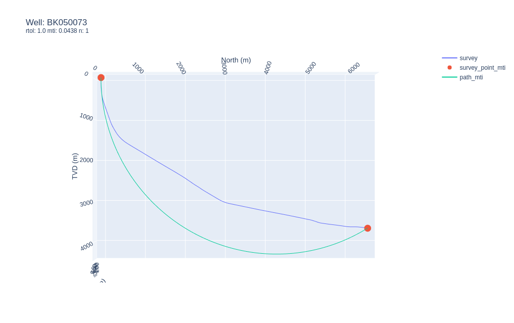Synthetic survey for well BK050073 with rtol=1.0.

Well this is unexpected! It appears that our ERD well approximates to a single constant build curve turn with a low MTI value of 0.0438 if we use the coarse rtol=1.0 parameter. Clearly for this well, using such a coarse rtol value results in an over-approximation and under-states the MTI value.

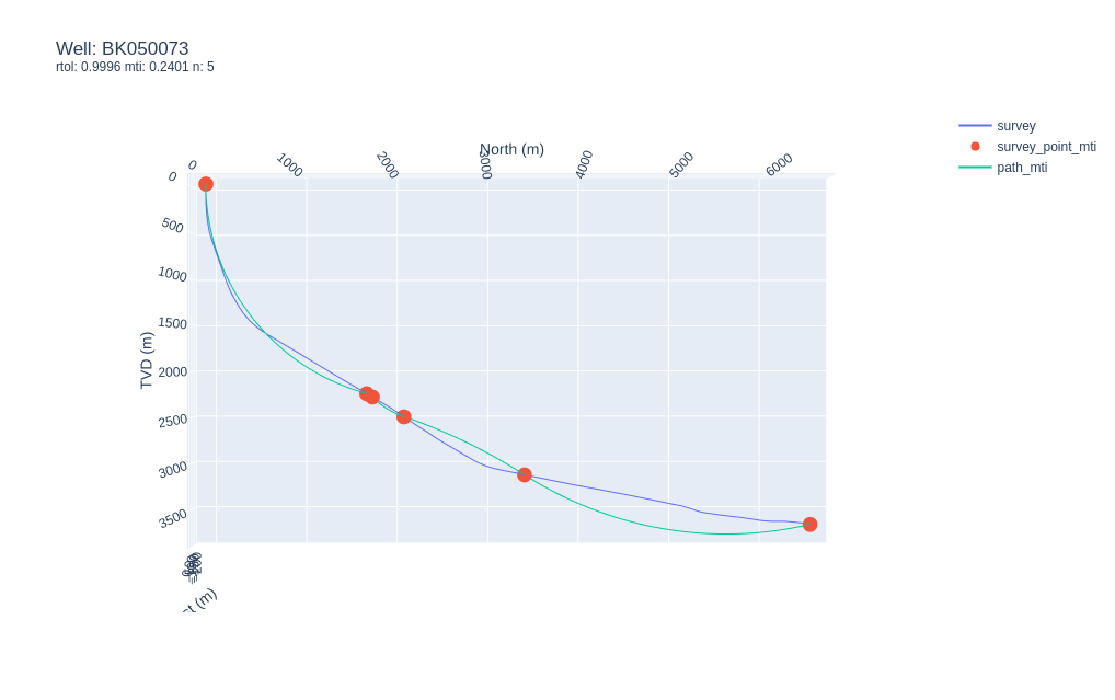Synthetic survey for well BK050073 with rtol=0.9996.

Reducing the rtol parameter by as little as 0.0004 to rtol=0.9996 returns a much tighter approximation with a resulting higher MTI value of 0.2401, but still it doesn’t really honor all the features of the drilled trajectory.

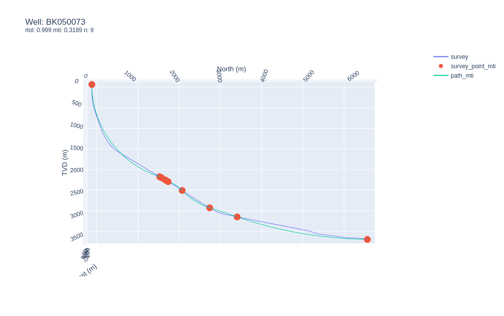Synthetic survey for well BK050073 with rtol=0.999.

Again, reducing the rtol parameter to rtol=0.999 adds another 4 control points and bumps up the MTI value again to 0.3189, providing a visually tighter fit to the as-drilled survey trajectory, but there’s still a noticeable difference.

Synthetic survey for well BK050073 with rtol=0.1.

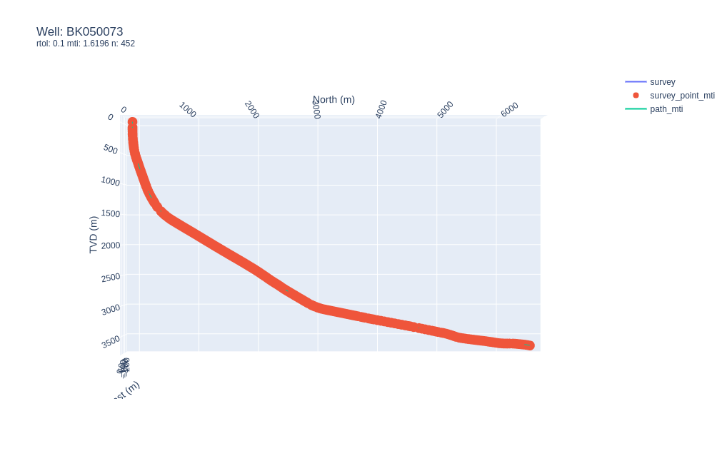
This time the rtol parameters has been dropped right down to rtol=0.1 which results is a very tight fit to the survey trajectory and a high MTI value of 1.6196, at the cost of many more sections, reducing the survey sections from 567 to 452 which means that only a few sections are considered continuous.

So, what rtol value should we be using for calculating the MTI? Clearly some more analysis is required.

Tolerance Analysis

Let’s write some code so we can compare a range of MTIs versus rtols:

# construct a range of rtol values, weighted in the range 0.9 to 1.0
rtols = np.hstack((
    np.linspace(0.001, 0.9, 1000, endpoint=False),
    np.linspace(0.9, 1.0, 1000)
))

mtis = [
    survey.modified_tortuosity_index(rtol=rtol)[-1]
    for rtol in rtols
]

# construct a figure
fig_mtis = go.Figure()
fig_mtis.add_trace(
    go.Scattergl(
        x=rtols,
        y=mtis
    )
)

fig_mtis.add_vrect(
    x0=0.1, x1=0.4, line_width=0, fillcolor="red", opacity=0.2
)

fig_mtis.update_layout(
    title=(
        f"Well: {survey.header.name}"
        f"<br><sup>MTI versus rtol</sup>"
    ),
    xaxis=dict(
        type='log',
        title='rtol'
    ),
    yaxis=dict(
        title='MTI'
    )
)

with the console command fig_mtis.show() the following chart should pop up in a web browser:

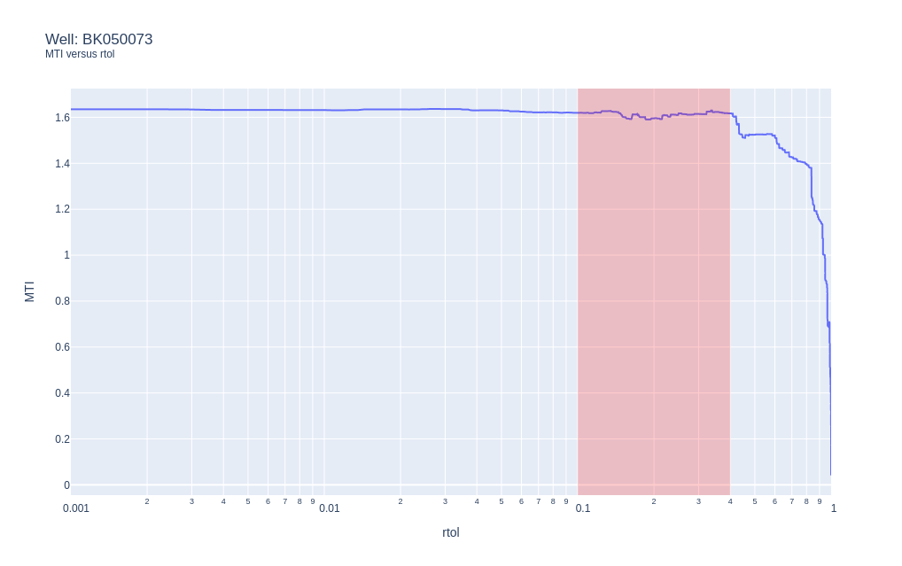MTI versus rtol for well BK050073.

The chart indicates that for rtol values below 0.1 that the MTI results are pretty constant with a little bit of instability between 0.1 and 0.4 and a drop off in MTI values above rtol values of 0.4. This indicates that for as-drilled surveys for well trajectories, the maximum rtol value should be set around 0.1 to appropriately capture as-drilled tortuosity, but that a default value of 0.01 should be considered to steer clear of the instability and promote consistent results.

Dogleg Severity (DLS) Continuity

Until now and to remain consistent with the University of Texas Tortuosity Index method, we have not considered continuity of the DLS as it has been assumed that rate of curvature does not impact tortuosity. Personally, I do not agree with this assumption and the mental analogy I refer to is generally that of a roller-coaster ride - if I were to ride a roller-coaster would I feel a change in the radius of curvature of the track? I most definitely would as an increase in the rate of curvature would exert a larger force on my body, so it’s not unreasonable to assume that variations in curvature, even in the same plane, will exert undesirable forces on an assembly being run in a well bore.

First, let’s modify our continuity code so that we can determine dls continuity:

import numpy as np

# survey is a welleng.survey.Survey instance

# accommodate scenario where we're not interested in dls continuity
if dls_tol is None:
    dls_continuity = np.full(len(survey.dls) - 2, True)

# otherwise, check for continuity of successive section dls values within a
# defined tolerance `dls_tol` parameter.
else:
    dls_continuity = np.isclose(
        survey.dls[1:-1],
        survey.dls[2:],
        equal_nan=True,
        rtol=dls_tol,
        atol=rtol
    )

# now we can consider dls_continuity as well as normal vector continuity
continuous = np.all((
    np.all(
        np.isclose(
            survey.normals[:-1],
            survey.normals[1:],
            equal_nan=True,
            rtol=rtol, atol=rtol
        ), axis=-1
    ),
    dls_continuity
), axis=0)

In the above code, the dls_tol parameter (in degrees per 30m) is the maximum difference that we’ll accept to consider the dls being constant between two successive sections. For example, if dls_tol=0.5, \(dls_{1} = 2.0\) and \(dls_{2} = 2.3\), then the dls_continuity will be determined as True since the values are within the dls_tol parameter, i.e.:

\[\left\lvert dls_{2} - dls_{1}\right\rvert \le dls_{tol}\]

For the case where rtol=1.0, let’s plot MTI versus a range of dls_tol values and include the number of curve-turn or hold sections:

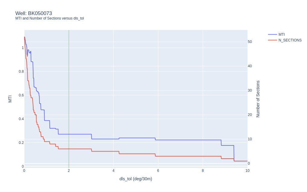MTI and the Number of Sections versus \(dls_{tol}\) for well BK050073.

The results indicate that for \(8 > dls_{tol} > 2\) the MTI and number of sections is relatively constant and that for \(dls_{tol} < 2\) the MTI and number of sections ramps up quickly. For \(dls_{tol} > 10\) there’s no significant difference versus simply ignoring the dls continuity.

These results suggest that there is merit in taking account of dls continuity for higher rtol values and that dls_tol=2.0 is a suitable default parameter value.

Let’s redraw the chart where rtol=1.0 but this time include our dls_tol=2.0 parameter and check for dls continuity:

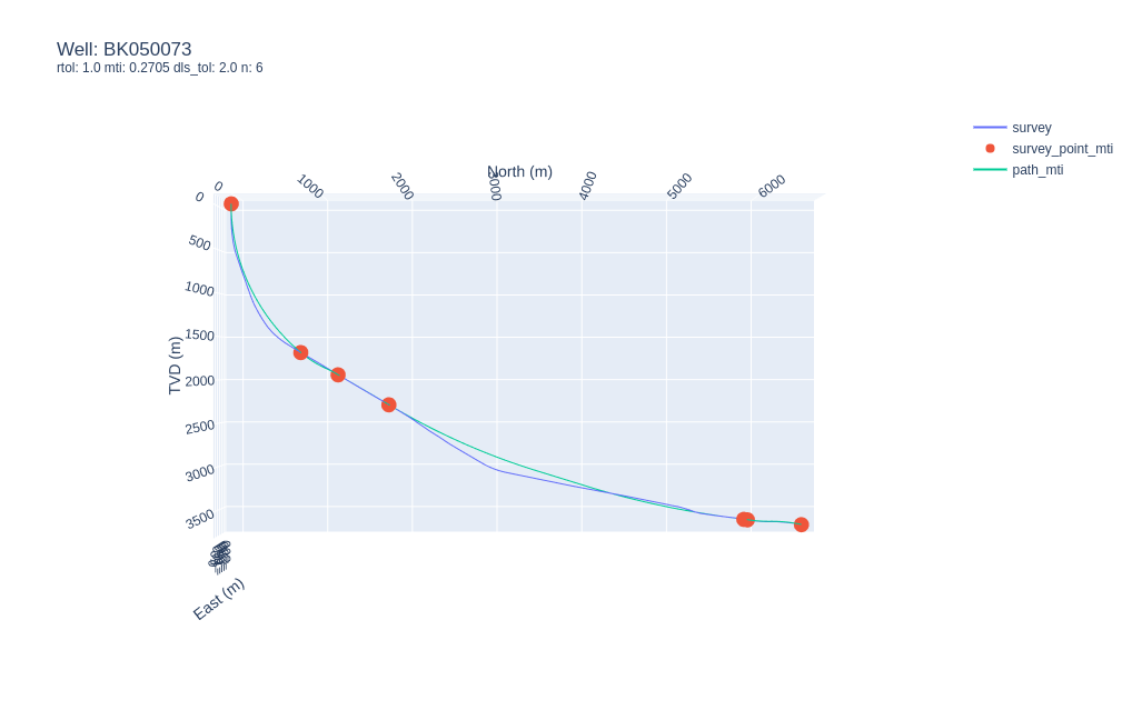Synthetic survey for well BK050073 with rtol=1.0 and dls_tol=2.0.

This is a markedly better fit to the as-drilled trajectory while maintaining a minimal number of sections - it’s a pretty good approximation of what the planned well trajectory may have looked like, the significance of which is described below.

Well Bore Quality

The University of Texas team have described previously methods for assessing as-drilled surveys versus planned surveys. What if we didn’t need the planned survey in order assess directional drilling performance?

Above we’ve determined parameters for rtol and introduced a dls_tol parameter and default such that we can now confidently and consistently calculate a robust MTI value for an as-drilled well. But we’ve also developed a method of distilling an as-drilled trajectory down to a minimal number of sections that can represent the planned well trajectory, adequate enough to give a realistic baseline MTI value as a proxy for the planned trajectory.

Well bore quality could now defined as:

\[QI_{tortuosity} = \left(\frac{MTI_{drilled}}{MTI_{planned}} - 1\right)\]

Where \(MTI_{drilled} > MTI_{planned}\) and larger \(QI_{tortuosity}\) values indicate increasing tortuosity relative to the planned trajectory versus the absolute MTI value.

So for our BK050073 example well, using rtol=0.01 and dls_tol=2.0 we get \(MTI_{drilled} = 1.63\) and using rtol=1.0 and dls_tol=2.0 we get \(MTI_{planned} = 0.27\). If we substitute these values into the above equation we get \(QI_{tortuosity} = 5.03\).

The result seems too high - previous experience leads me to think that the range of values for the MTI should be in the range of 0.0 to 1.0 and this result is significantly higher than this, so let’s take a closer look by plotting the delta MTI between survey stations.

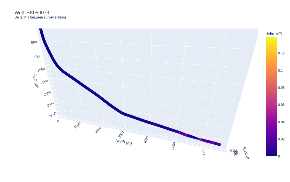Survey for well BK050073 with rtol=0.01 and dls_tol=2.0 and colored on the delta MTI between survey stations.

As we’d expect, the delta value between survey stations is quite consistent along the trajectory until around 7,476 mMD where there’s a relatively high value (colored in yellow in the above figure). Inspection of the survey data at this depth indicates that there’s a relatively large DLS of 8 deg/30m.

Plotting the MTI versus depth also indicates a steep increase in tortuosity towards the TD of the well trajectory, driving up the MTI value.

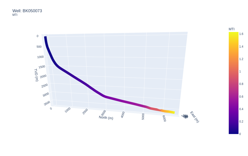Survey for well BK050073 with rtol=0.01 and dls_tol=2.0 and colored MTI.

Above illustrates a process for quickly identifying tortuous well trajectories and finding where along the well path any local tortuosity occurs. Let’s quickly review the entire NLOG database:

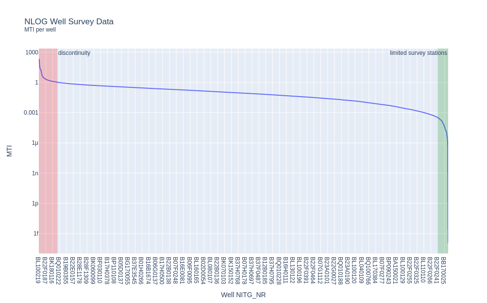NLOG well MTI values sorted in descending order (y-axis is log scale).

Of note here is that the majority of the MTI values lie in the range 0.001 to 1.0. Closer examination of the wells with high MTI values (the red area in the above figure), using the method outlined above are revealed to have discontinuities (very high MTI values) or high dog legs (lower MTI values in the red band).

Specifically for the high value MTI wells:

NITG_NR wells BP050076, BL100169, BL100219 are missing azimuth data.
NITG_NR well BL080112 azimuth is wrong at 4352 mMD (should probably be 252.3 degrees).
NITG_NR well BK120155 final survey station is likely wrong.
NITG_NR well B19B0267 has a couple of abrupt azimuth changes, e.g. at 920 mMD. It also appears that this survey has been interpolated.
NITG_NR well B11B0050 has an abrupt inclination and azimuth change at 2270.2 mMD.

Of the green banded results with low MTI values, there are either insufficient survey stations to calculate the MTI (typically only two stations, one at surface and one at the well TD) yielding a NaN value which is represented here as zero, else the survey has a low number of survey stations, which brings us onto survey station frequency.

Survey Station Frequency

There’s one more variable that has a large influence on \(MTI_{drilled}\) which can also influence the \(QI_{tortuosity}\) value and that is the frequency of the survey stations, or the distance between each survey station.

Because we generally use the minimum curvature method to coerce a trajectory between two survey stations, we always under-estimate the actual well bore tortuosity. Typically for an MWD survey, the variance in DLS over the calculated DLS can be around 0.5-1.0 deg/30m. For sparse surveys, this underestimate of tortuosity is exaggerated which yields a relatively low MTI value for a drilled survey which we need to address if we want to use the MTI and \(QI_{tortuosity}\) values as generic indications of as-drilled well tortuosity and quality metrics.

A standard method to apply tortuosity variance onto a survey will be the topic of a future post.

Conclusions

The MTI and \(QI_{tortuosity}\) remain useful tools for defining and comparing the tortuosity of a well path and as a quality indication versus a planned or reference trajectory design. However, care must be taken to use appropriate tolerances when checking for curve and DLS continuity. Further, sparsely populated surveys (long distances between survey stations) result in misleading low MTI and \(QI_{tortuosity}\) results, which needs further investigation.

Further testing and refinement is required and recommended before applying this method.

As usual, please feel free to leave any comments or feedback.