A Modified Tortuosity Index

Summary

The Drilling Tortuosity Index (TI) is a useful method for determining the relative complexity of a well trajectory and as a Key Performance Indicator (KPI) when assessing well quality.

This post describes the Modified Tortuosity Index (MTI) that proposes modifications to the Tortuosity Index to make it inherently three-dimensional and dimensionless and provides details and data on how to apply the method using the Python library welleng.

Disclaimer

The following method is experimental and has yet to be thoroughly tested - the work presented is that of an enthusiastic amateur, with no professional or otherwise affiliations. As such, please use with caution and do your own research and testing - the only request is that, in the spirit of open source you report back your own findings either via the comments below or via the welleng repository. The license is permissive - the only requirement is that you reference the source if you use the method or code.

Background

The Tortuosity Index method that is generally used in the Drilling community is derived from the medical industry. This method was adapted and developed for well trajectories by Pradeep Ashok et al at The University of Texas and presented at the International Association of Directional Drilling. Several SPE papers on the subject have subsequently been published.

The generally accepted equation for the drilling Tortuosity Index (TI) is:

\[TI_{inc/azi} = \frac{n}{n + 1} \frac{1}{L_{c}}\sum_{i = 1}^{n}\left(\frac{L_{csi}}{L_{xsi}} - 1\right)\] \[TI_{3D} = \sqrt{\left(TI_{inc}\right)^{2} + \left(TI_{azi}\right)^{2}}\]

where n is the number of curve turns, L_csi is the arc length of the curve turn, L_xsi is the chord length of the curve turn and L_c is the total curve length.

The method states that calculating the TI for the curvature in the inclination and azimuth domains enables the three dimensional TI_3D to be calculated by taking the root of sum of the squares of the TI_Incl and TI_Azm. For this to hold, when calculating TI_Incl and TI_Azm, only the inclination and azimuth components of the curves should be considered for L_csi, L_xsi and L_c, else TI_Incl and TI_AZM are not independent and as such, the current application of the TI is not mathematically correct, although whether this is practically significant is out of scope here.

Definition of a Curve Turn

The presentation does a good job of describing a two-dimensional curve, but what if we can skip trying to merge two two dimensional curves and consider a curve turn directly in three-dimensions?

When planning and drilling wells these days, we almost exclusively use the minimum curvature method, which is essentially an arc path on the surface of a plane in three-dimensional space.

Curve turn of a well trajectory: a continuous curve turn between points A and B occurs along a plane surface. The normal vectors of the plane \(norm_{A} == norm_{B}\) are represented by the blue arrows, the initial trajectory vector \(vec_{A}\) by the green arrow and the final trajectory vector \(vec_{B}\) the red arrow. Note that the normal vectors have been flipped to make the figure look better, but the principle holds.

With reference to the above figure, given the unit vectors of the well trajectory at points A and B, the normal vector of the plane can be determined by the cross product of \(vec_{A}\) and \(vec_{B}\):

\[norm = vec_{A} \times vec_{B}\]

Interestingly, the normal vectors are not effected by radius of curvature of the turn (or the dog leg severity), which aligns with the standard TI methodology of defining curve turns.

Generate a Well Trajectory

Now that we’ve established that the normal vectors at any point along a curve turn are identical, we can use this feature to determine the number of curve turns and the associated arc and curve lengths.

We need a simple well trajectory to try it out, so we’ll quickly generate the ISCWSA standard well trajectory number 1:

import numpy as np
import welleng as we


# survey header data
sh = we.survey.SurveyHeader(
    name="ISCWSA No. 1: North Sea extended reach well",
    latitude=60,
    longitude=2,
    G=9.80665,
    b_total=50_000,
    dip=72,
    declination=-4,
    vertical_section_azimuth=75,
    azi_reference='magnetic'
)

# generate survey
md, inc, azi = np.array([
    [0.0, 0.0, 0.0],
    [1200.0, 0.0, 0.0],
    [2100.0, 60.0, 75.0],
    [5100.0, 60.0, 75.0],
    [5400.0, 90.0, 75.0],
    [8000.0, 90.0, 75.0]
]).T

survey = we.survey.Survey(
    md, inc, azi,
    header=sh
).interpolate_survey(step=30)

We can quickly QAQC the trajectory with the following convenience method:

>>> survey.figure().show()

This generates the following Plotly chart:

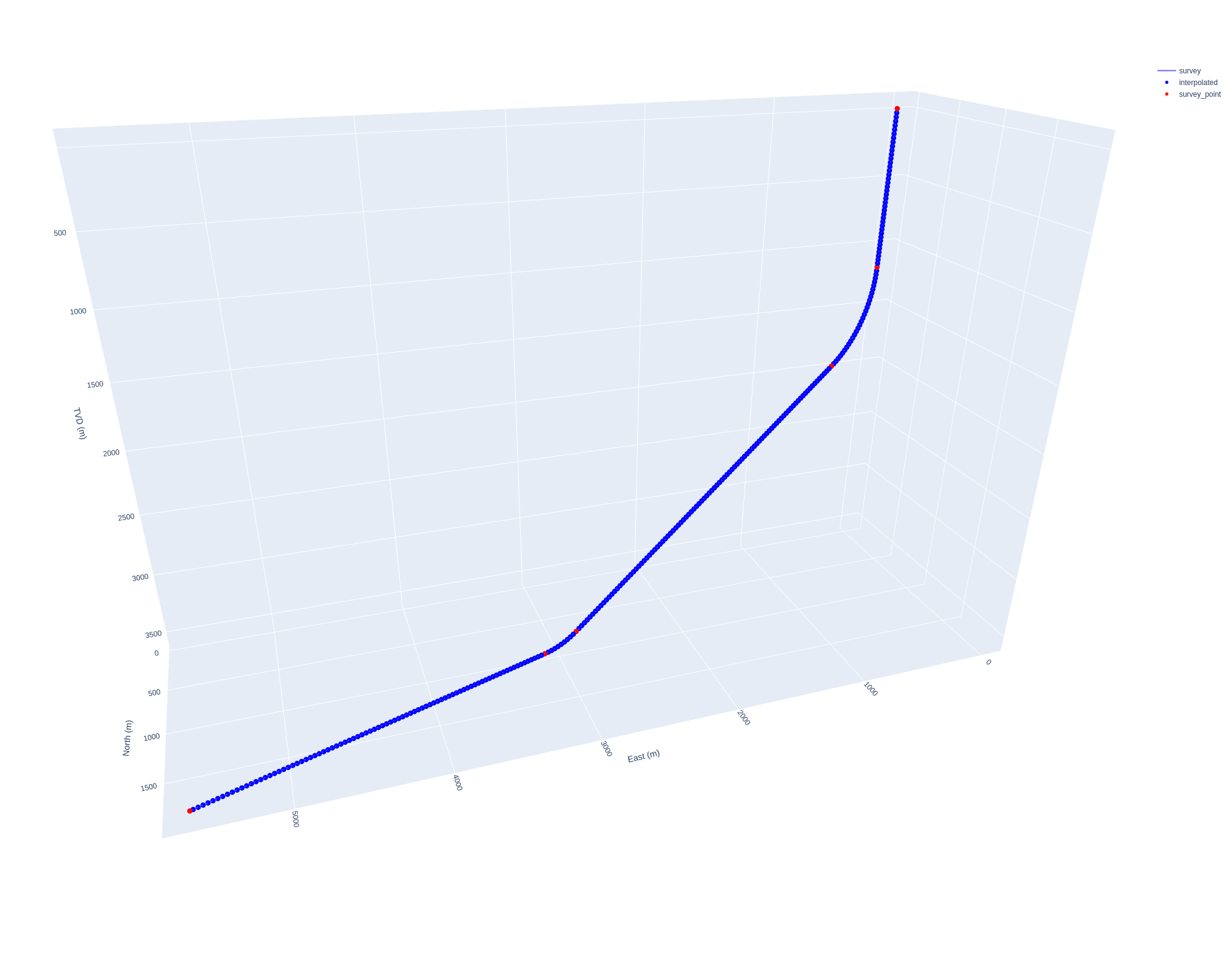ISCWSA Standard Well Trajectory Number 1

Calculate the Normals

In order to split the well into sections, we’ll need to determine the normals. This is made simple with welleng as it’s already calculated and a property of the Survey instance:

>>> survey.normals

Reviewing the array of normal vectors reveals that for the tangent sections of the well there are no normal vectors on account of there being no solution to a cross product of identical vectors. This is a useful result as it allows us to include these tangent sections as discrete curve turns (with infinite radius) where the arc length is equal to the chord length.

Below is a plot of the well path with the curve turn normals added:

ISCWSA Standard Well Trajectory number 1 with the curve turn normal vectors indicated in blue: note how the normal vectors are identical/aligned throughout each curve indicating continuity.

Determine the Trajectory Sections

The lack of normal vectors on the remainder of the well path indicates hold sections and therefore the well consists of 5 sections:

Section 1: a vertical hold section
Section 2: a build section
Section 3: a tangent hold section
Section 4: a build to align to target
Section 5: a hold to target

With the normals calculated, we can now iterate through them in order to determine curve turn and hold sections. This is comparing the normal vector of node n + 1 with the previous normal vector of node n.

With Python, this can be achieved with the following code, where survey is a welleng Survey instance with a normals property:

import numpy as np


continuous = np.all(
    np.isclose(
        survey.normals[:-1],
        survey.normals[1:],
        equal_nan=True
    ), axis=-1
)

The above could also be implemented with Python’s built in functions, but it’s simpler (and possibly faster for larger surveys) to use numpy which achieves the operation in a single line of code. For transparency, it’s worth walking through what the operation is doing.

The survey.normals are being split into two lists which represent the point A and point B nodes, i.e. pairs of adjacent trajectory stations.
We mentioned earlier that there’s no solution to a cross product of two identical vectors (or rather there’s an infinite number of solutions), which means that for hold sections of the trajectory, the normal vectors are [nan, nan, nan] (i.e. a 1,3 matrix of not a number). Since these are not numbers, we need to provide an instruction on how to deal with these, so the parameter equql_nan states that if there’s a pair of nans then we treat them as being equal to each other.
Now we have the requisite parameters for the numpy.isclose function, which “Returns a boolean array where two arrays are element-wise equal within a tolerance” - note: we’ve not provided a tolerance in this example because it’s a planned trajectory with precise numbers, but for as drilled surveys the likelihood of two sections being continuous with the default tolerance values is practically zero, but we’ll discuss this later.
The result of the numpy.isclose function is an (n,3) boolean aray (i.e. [True, True, True] of the pairs of normal vectors), but we’re interested in the whether all of the elements are equal so we use the numpy.all function to check each boolean matrix and see if all three values are True - the axis=-1 parameter instructs the function to check row-wise, i.e. a single boolean for each pair of normal vectors.

The above operations are summarized in the flowchart below:

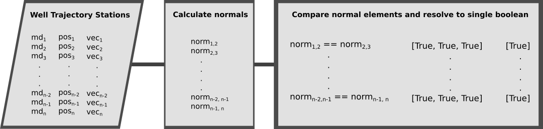Flowchart describing the process of determining a well path’s curve turn continuity from its vectors (inclination and azimuth) - continuity is considered true when the elements of a survey station’s normal vector are all equal to the normal of the previous survey station’s normal vector.

We now have a one-dimensional boolean array which we can index against the survey and for each survey station and determine if it continues the current curve turn or hold section. Where the continuity array is False indicates the end of the curve turn or hold section and the start of a new one, so counting the number of False elements in the array indicates the number of sections in the well, which is the n value in the TI equation.

Systematically taking the index of the False values in the continuity array, we can find the position and the measured depth at the end of each curve turn or hold section and use these values to calculate the L_c, L_ci and L_xi values in the TI equation in the knowledge that they’re now mathematically robust numbers.

In Python we can do all this quite succinctly with numpy:

# get the indexes of the survey stations at the start of each curve turn or
# hold section - manually add the first index at 0.
starts = np.concatenate((
        np.array([0]),
        np.where(continuous == False)[0] + 1,
    ))

# using this index, get the md and pos of these start stations
mds = survey.md[starts]
locs = survey.pos_nev[starts]

# make an array of the number of sections and use it to assign a section
# number for each survey station - e.g. station 5 is in section 1
n_sections = np.arange(1, len(starts) + 1, 1)
n_sections_arr = np.searchsorted(mds, survey.md[1:])

# with the above we can calculate l_cs and l_xs
# l_cs is the current section start to the current station
l_cs = (survey.md[1:] - mds[n_sections_arr - 1])

# l_xs is the straight line distance from the section start pos to the current
# station pos
l_xs = np.linalg.norm(
    survey.pos_nev[1:]
    - np.array(locs)[n_sections_arr - 1],
    axis=1
)

Note: when calculating L_cs and L_xs for each survey station, we need to reference the md and pos at the beginning of the current curve turn or hold section respectively, which is why there’s some funky indexing going on above.

Modified Tortuosity Index (MTI)

The current TI is not dimensionless and the reference TI ranges are expressed in ft^-1. The Modified Tortuosity Index (MTI) proposes a tweak to the equation to make it dimensionless - results from surveys in feet can be compared directly to those from surveys in meters (or any other unit):

\[MTI_{n} = \frac{n}{n + 1} {\kappa}{L_{c}}\sum_{i = 1}^{n}\left[\left(\frac{L_{csi}}{L_{xsi}} - 1\right) \times \frac{1}{L_{csi}}\right]\]

Where \(\kappa\) is a constant for which 1 seems to be appropriate, but I’ve left this in since in the reference TI equation this value is \(1\times{10^{7}}\) which is easily overlooked. Note that the \(\frac{1}{L_{csi}}\) product has been added in the summation and the \(L_{c}\) term is no longer an inverse, the intent of which is to make the MTI result dimensionless.

The next step is not intuitive (to me at least) as the summations need to be done per section. I’m not completely sure that the above equation correctly represents this, but I can express it in Python code:

# set the value for the constant kappa
kappa = 1.0

# start by calculating the bracketed terms in the summation except for the
# Lci term which needs more attention
b = (
    (l_cs / l_xs) - 1
) / (l_cs)

# with a for loop, iterate through each section, adding the last result of the
# previous section - this enables the MTI to be calculated for all stations
# along the well trajectory and is the value of the summation in the equation
cumsum = 0
a = []
for n in n_sections:
    a.extend(
        b[n_sections_arr == n]
        + cumsum
    )
    cumsum = a[-1]
a = np.array(a)

# calculate the mti as per the equation
mti = np.hstack((
    np.array([0.0]),  # manually add the first value
    (
        (n_sections_arr / (n_sections_arr + 1))  # n / n + 1
        * (kappa * (survey.md[1:] - survey.md[0]))  # kappa * Lc
        * a  # the summation
    )
))

And there you have it, the Modified Tortuosity Index (MTI).

Let’s write a bit more code to visualize the result:

# generate a plot to show MTI using the figure method to initiate a plotly
# chart
fig = survey.figure()

# hide the survey points data
for i in range(1, 3):
    fig.data[i].visible = False

# color the well trajectory with the mti values, make the line thicker and add
# a colobar to show the mti values
fig.data[0]['line']['color'] = mti
fig.data[0]['line']['width'] = 20
fig.data[0]['line']['colorbar'] = dict(
    thickness=40, title="MTI"
)

# add a title
fig.update_layout(
    title="Modified Tortuosity Index (MTI)<br><sup>ISCWSA Example no. 1</sup>"
)

To show the figure, use the following command:

>>> fig.show()

The following plotly figure should pop up in your web browser:

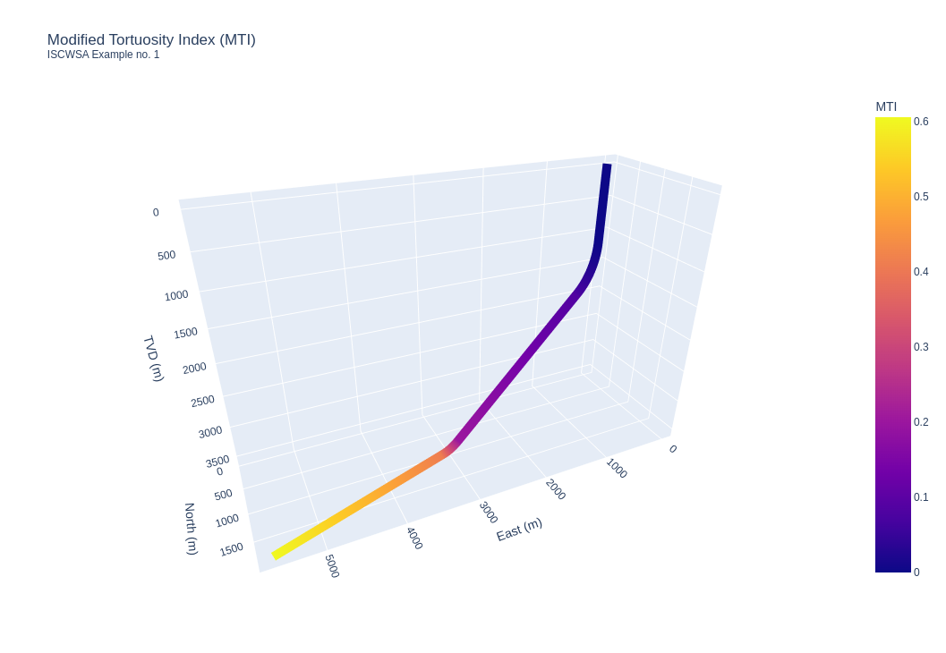ISCWSA Standard Well Trajectory Number 1 colored with MTI values

Tolerances and Station Frequency

As eluded to earlier, in an actual well survey (versus a planned survey), it is probable that the normal vectors of consecutive stations are not exactly equal, which will result in a highly discontinuous well trajectory. Further, the md interval between the trajectory stations (station frequency) is likely less regular for an as drilled well versus a planned well with e.g. a station every 30 meters or 100 feet.

It’s simple enough to add a tolerance to the numpy.isclose function that is used in welleng to calculate the continuity and the default welleng rtol and atol values are surprisingly coarse at 1.0 each, i.e. when subtracting the normal elements from one another, values less than 1.0 are considered close and return a True boolean. What this practically means is that we’re really checking for sign changes in the normal vectors, i.e. switching from up to down or from left to right - some future optimization here may be warranted.

Diagnostic Data

The intent of this post is describe and walk through the implementation of the Modified Tortuosity Index so that it can be peer reviewed, replicated and tested. Diagnostic data is in json format for the worked examples is available here to be used as diagnostic data for testing out your own implementation.

Here’s the code for extracting the data from the survey and saving it to a json format:

import json

# extract data from the survey and include the mti results
data = {
    'header': vars(survey.header),
    'data': {
        i: {
            'md': md, 'inc': inc, 'azi': azi, 'northing': n,
            'easting': e, 'tvd': tvd, 'vec': vec.tolist(),
            'norm': norm.tolist(), 'mti': mti
        }
        for i, (md, inc, azi, n, e, tvd, vec, norm, mti)
        in enumerate(zip(
            survey.md, survey.inc_deg,
            getattr(
                survey,
                f"azi_{survey.azi_ref_lookup[survey.header.azi_reference]}_deg"
            ),
            survey.n, survey.e, survey.tvd, survey.vec_nev, survey.normals,
            mti
        ))
    }
}


def round_em_off(data, decimals=3):
    """
    A quick function to round off the data, ignoring the matrices.
    """
    temp = {}
    for k, v in data.items():
        if isinstance(v, list):
            temp[k] = v
        else:
            temp[k] = np.round(v, decimals)

    return temp


# round off the numbers
for row in data['data']:
    data['data'][row] = round_em_off(data['data'][row])

# save to file in json format
with open('iscwsa-example-1-mti.json', 'w') as fp:
    json.dump(data, fp)

Alternatively, you can use the welleng library (version >= 0.4.10) to generate your own diagnostic data as per the following example with the ISCWSA Example no 2 well trajectory:

import numpy as np
import welleng as we


# ISCWSA No. 2
# survey header data
header = we.survey.SurveyHeader(
    name="ISCWSA No. 2: Gulf of Mexico fish-hook well",
    latitude=28,
    longitude=-90,
    G=9.80665,
    b_total=48_000,
    dip=58,
    declination=2,
    vertical_section_azimuth=21,
    azi_reference='true'
)

# generate survey array - these are in feet
md, inc, azi = np.array([
    [0.0, 0.0, 0.0],
    [2000.0, 0.0, 0.0],
    [3600.0, 32.0, 2.0],
    [5000.0, 32.0, 2.0],
    [5525.54, 32.0, 32.0],
    [6051.08, 32.0, 62.0],
    [6576.62, 32.0, 92.0],
    [7102.16, 32.0, 122.0],
    [9398.5, 60.0, 220.0],
    [12500.0, 60.0, 220.0]
]).T

# initiate Survey instance
survey = we.survey.Survey(
    md * 0.3048,  # convert to meters
    inc, azi,
    header=header
).interpolate_survey(step=100 * 0.3048)  # convert per 100 ft to meters

# calculate the MTI using the convenience method
mti = survey.modified_tortuosity_index()

# check the result
# generate a plot to show MTI
fig = survey.figure()

for i in range(1, 3):
    fig.data[i].visible = False

fig.data[0]['line']['color'] = mti
fig.data[0]['line']['width'] = 20
fig.data[0]['line']['colorbar'] = dict(
    thickness=40, title="MTI"
)
fig.update_layout(
    title="Modified Tortuosity Index (MTI)<br><sup>ISCWSA Example no. 2</sup>"
)

Running the above code will generate the following plotly figure:

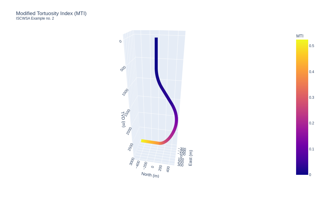ISCWSA Standard Well Trajectory Number 2 colored with MTI values

Conclusion

The Modified Tortuosity Index (MTI) is a dimensionless and natively three-dimensional method for determining a Tortuosity Index for a well trajectory (or any other sort of trajectoy or path). For the wells and drilling domain, the welleng library includes convenient methods for quickly generating the MTI, and code and diagnostic data is included in this post to facilitate testing, verification and further development.

Further testing and refinement is required and recommended before applying this method.

As usual, please feel free to leave any comments or feedback.