Gravity Battery Potential in the Netherlands
Following on from the previous post that presented the Gravity Well as an energy storage concept, some further digging determined that the potential energy storage capacity using existing wells located in the Netherlands is 480 MWh.
This post will describe how this number was derived and conclude with some perspective.
Data Source
We’ll be using the NLOG Dutch Oil and Gas Portal to get data on the in-situ wells in the Netherlands. The data includes an overview of the wells and the survey listing for each well, but unfortunately does not include casing geometry (casing sizes and depths).
An overview of the wells is available here as a Microsoft Excel .xls file - which can be loaded directly into a pandas DataFrame. This helper function avoids having to save the file locally to your computer:
import requests
from io import BytesIO
import pandas as pd

def get_file_data(url):
    '''
    Function to download a file to memory from a url
    '''
    response = requests.get(url)
    f = BytesIO()
    for chunk in response.iter_content(chunk_size=1024):
        f.write(chunk)
    f.seek(0)
    return f
The summary DataFrame can be created with the following:
url_summary = 'https://www.nlog.nl/nlog/queryAllWellLocations?menu=act&ACT_DOWNLOAD_RESULT=true&all=true'

df_summary = pd.read_excel(get_file_data(url_summary))
Getting the deviation data imported was more challenging, since for some reason NLOG choose to distribute this data as an .xlsx file which is not well supported these days due to security concerns. The easiest option ended up being to download it and use LibreOffice Calc or similar to export the data as a .csv file. It is possible to import the data with openpyxl but it loads really slow (even with read_only=True).
If anyone from NLOG is reading this, please consider distributing the data in a more versatile format - even
.csvwould be preferable over Closed Source Software output data.
The deviation data can then be read into another pandas DataFrame.
df = pd.read_csv(file_deviation)
where file_deviation is the path and filename of the local .csv file exported from the spreadsheet application.
Filtering the Data
Now that the data has been imported, it needs to be filtered.
For now, we’re only interested in onshore wells as these would be the simplest to convert to energy storage and hook up to the grid. The well names can be filtered using the summary data, which has a column indicating wether the well is on or offshore.
Since we don’t know the geometry of these wells, we’ll make an assumption that the available drift is 8 1/2 inches, i.e. that we have access to a 9 5/8” production casing - not an unreasonable assumption for the deeper wells that we’re interested in and based on experience with NAM wells. Based on the previous post, we’re looking for True Vertical Depths (TVD) of at least 2,000 meters for wells with an 8 1/2 inch drift.
The final filter we’ll apply is on the inclination. We’ll make an assumption that we only want to run the mass inside well bores that remain below 5 degrees.
These depth and inclination filters are applied to the deviation data and these wells cross-referenced with the onshore wells from the first filter.
There are 6,562 wells listed by NLOG, of which 4,413 are indicated as being located onshore. When we filter with our minimum depth and inclination constraints, we’re left with 376 wells that we can be reasonably confident about converting to gravity wells.
Calculating Storage Capacity
Using the code from the previous post we can calculate the peak power and capacity for each of our 376 wells. For the depth of each well, we use the depth at which the well bore inclination first deviates above 5 degrees, else we assume that the well is vertical for the entire length.
Once we’ve calculated these, we can lookup each well’s surface location and plot it on a map, color coding the marker to indicate its storage capacity.
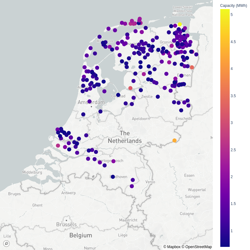 Potential electrical storage capacity in the Netherlands through the conversion of existing oil and gas wells to gravity storage wells.
If we now sum up across our wells, we reach 487 MWh of potential storage capacity, with a combined peak output of 197 MW.
Context
Let’s take a look at the total renewable energy production in the Netherlands over the last decade, which in 2018 accounted for 15% of the total electricity consumption of the country.

Renewable energy production in the Netherlands from CBS.
If we only consider wind and solar (since these are the unpredictable producers that necessitate energy storage), in 2018 the Dutch generated 13 billion kWh. Let’s first align units - 13 billion kWh is 13 million MWh and is the production over the entire year. For simplicity, we’ll convert this to an average daily production of 35,616 MWh.
So on average, our 376 gravity wells have the capacity to store 1.3% of the average solar and wind electricity production of the Netherlands.
Conclusion
I shall leave you to make your own conclusions.