Connection Conundrums - Part 4
In part 3 we used our network graph to determine all of the permutations of casing designs that can be generated with the Tenaris Wedge 521 connections range. We observed that from these 92 casing connections we can produce over 5 million unique casing designs and that using networkx which is written in Python code and despite multiprocessing with ray.
In this post, we’re going to switch to a faster implementation of network graphs that utilizes C/C++ in the back-end and stores the attributes as [numpy] arrays which will allow us to efficiently filter our nodes and generate sub-graphs only containing the nodes that our relevant for our application.
Introducing graph-tool
We’re going to quickly step through setting up a graph-tool network graph, which requires a bit more effort than for networkx, which in this case is the price we way for the performance boost.
Installation instructions can be found here and since I generally use conda environments for developing Python code, installing graph-tool is a relatively straight forward terminal command inside my connections env:
conda activate connections
conda install -c conda-forge graph-tool
Note that the connections env here is pretty fresh - it’s recommended (also in the installation instructions) to create a new env to mitigate the risk of the installation failing.
Importing libraries and data
We’ll start by copying and slightly modifying our code from part 2, changing from networkx to graph-tool. The Counter class is no longer required.
import numpy as np
import graph_tool as gt
import import_from_tenaris_catalogue  # our code from part 1

def make_graph(catalogue):
    # Now we want to initiate our graph - we'll make the edges directional, i.e.
    # they will go from large to small
    graph = gt.Graph(directed=True)

    return graph
Make some vertices
It’s time to add our nodes (called a vertex or vertices in graph-tool, so we’ll align with this from now on) and we come to one of the main differences between graph-tool and networkx - vertex and edge attributes need to be configured and typed beforehand with graph-tool and the data is handled as indexed arrays rather than Python dictionaries that are attributed to individual nodes and edges.
Since this is not meant as a lesson on how to use graph-tool, I’m not going to explain what’s happening here, but I’ve commented in the code.
def add_vertices(
    graph, manufacturer, type, type_name, tags, data
):
    """
    Function for adding a node with attributes to a graph.

    Parameters
    ----------
    graph: Graph object
    manufacturer: str
        The manufacturer of the item being added as a node.
    type: str
        The type of item being added as a node.
    type_name: str
        The (product) name of the item being added as a node.
    tags: list of str
        The attribute tags (headers) of the attributes of the item.
    data: list or array of floats
        The data for each of the attributes of the item.

    Returns
    -------
    graph: Graph object
        Returns the Graph object with the additional node(s).
    """
    # when we start adding more conections, we need to be careful with indexing
    # so here we make a note of the current index of the last vertex and the
    # number of vertices we're adding
    start_index = len(list(graph.get_vertices()))
    number_of_vertices = len(data)

    graph.add_vertex(number_of_vertices)

    # here we initate our string vertex property maps
    vprops = {
        'manufacturer': manufacturer,
        'type': type,
        'name': type_name
    }

    # and then add these property maps as internal property maps (so they're)
    # included as part of our Graph
    for key, value in vprops.items():
        # check if property already exists
        if key in graph.vertex_properties:
            continue
        else:
            graph.vertex_properties[key] = (
                graph.new_vertex_property("string")
            )
        for i in range(start_index, number_of_vertices):
            graph.vertex_properties[key][graph.vertex(i)] = value

    # initiate our internal property maps for the data and populate them
    for t, d in zip(tags, data.T):
        # check if property already exists
        if t in graph.vertex_properties:
            continue
        else:
            graph.vertex_properties[t] = (
                graph.new_vertex_property("double")
            )
        # since these properties are scalar we can assign with arrays
        graph.vertex_properties[t].get_array()[
            start_index: number_of_vertices
        ] = d

    # overwrite the size - in case it didn't import properly from the pdf
    graph.vertex_properties['size'].get_array()[
        start_index: number_of_vertices
    ] = (
        graph.vertex_properties['pipe_body_inside_diameter'].get_array()[
            start_index: number_of_vertices
        ] + 2 * graph.vertex_properties['pipe_body_wall_thickness'].get_array()[
            start_index: number_of_vertices
        ]
    )

    # calculate and add our min and max pipe body burst pressures
    graph = add_burst_pressure_to_graph(graph)

    return graph
This time we’re going to consider pipe body burst pressure ratings to help us when selecting our casing connections, hence the reference to the function add_pipe_burst_pressure_to_graph(). This is a function for calculating the maximum and minimum ratings (based on the pipe body material grades ranging from 55 to 125 ksi) and adding this data to our Graph:
def calculate_pipe_burst_pressure(
    yield_strength,
    wall_thickness,
    pipe_outside_diameter,
    safety_factor=1.0
):
    burst_pressure = (
        (2 * yield_strength * 1000 * wall_thickness)
        / (pipe_outside_diameter * safety_factor)
    )

    return burst_pressure

def add_burst_pressure_to_graph(graph, yield_min=55, yield_max=125):
    attrs = ['pipe_burst_pressure_min', 'pipe_burst_pressure_max']
    for a in attrs:
        graph.vertex_properties[a] = (
            graph.new_vertex_property("double")
        )
    burst_min = calculate_pipe_burst_pressure(
        yield_strength=yield_min,
        wall_thickness=graph.vp['pipe_body_wall_thickness'].get_array(),
        pipe_outside_diameter=(
            graph.vp['pipe_body_inside_diameter'].get_array()
            + 2 * graph.vp['pipe_body_wall_thickness'].get_array()
        ),
        safety_factor=1.0
    )
    # lazy calculation of burst max - factoring the burt min result
    burst_max = (
        burst_min / yield_min * yield_max
    )
    # add the calculated results to our graph vertex properties
    for k, v in {
        'pipe_burst_pressure_min': burst_min,
        'pipe_burst_pressure_max': burst_max
    }.items():
        graph.vp[k].a = v

    return graph
Add some edges
Note that we’re already taking advantage of graph-tool’s utilization of arrays for storing vertex properties, also when determining our edges (which conections pass through which) in the code below:
def add_connection_edges(graph, cut_off=0.7):
    """
    Function to add edges between connection components in a network graph.

    Parameters
    ----------
    graph: (Di)Graph object
    cut_off: 0 < float < 1
        A ration of the nominal component size used as a filter, e.g. if set
        to 0.7, if node 1 has a size of 5, only a node with a size greater than
        3.5 will be considered.

    Returns
    -------
    graph: (Di)Graph object
        Graph with edges added for connections that can drift through other
        connections.
    """

    # get indexes of casing connections - we're thinking ahead since in the
    # future we might be adding more than just casing connections to our graph
    idx = [
        i for i, type in enumerate(graph.vp['type'])
        if type == 'casing_connection'
    ]

    # ensure that all the vertex properties exist - this list will likely
    # expand so at some point we might want a parameters file to store all our
    # property names that can be edited outside of this code
    vps = ['coupling_outside_diameter', 'box_outside_diameter']
    for vp in vps:
        if vp not in graph.vp:
            graph.vertex_properties[vp] = (
                graph.new_vertex_property("double")
            )

    # hold onto your seats... we're using array methods to do this super fast
    # calculate the clearance for every combination of connections
    clearance = np.amin((
            graph.vp['pipe_body_drift'].get_array()[idx],
            graph.vp['connection_inside_diameter'].get_array()[idx]
    ), axis=0).reshape(-1, 1) - np.amax((
        graph.vp['coupling_outside_diameter'].get_array()[idx],
        graph.vp['box_outside_diameter'].get_array()[idx],
        graph.vp['pipe_body_inside_diameter'].get_array()[idx]
        + 2 * graph.vp['pipe_body_wall_thickness'].get_array()[idx]
    ), axis=0).T

    # our data is raw and ideally needs cleaning, but in the meantime we'll
    # just ignore errors so that we don't display them to the console
    with np.errstate(invalid='ignore'):
        clearance_idx = np.where(
            np.all((
                clearance > 0,
                (
                    graph.vp['size'].get_array()[idx].T
                    / graph.vp['size'].get_array()[idx].reshape(-1, 1)
                    > cut_off
                )
            ), axis=0)
        )

    # make a list of our edges
    edges = np.vstack(clearance_idx).T

    # initiate an internal property map for storing clearance data
    graph.edge_properties['clearance'] = (
        graph.new_edge_property('double')
    )

    # add our edges to the graph along with their associated clearances
    # although we're not using this property yet, we might want to when
    # filtering our options later
    graph.add_edge_list(
        np.concatenate(
            (edges, clearance[clearance_idx].reshape(-1, 1)), axis=1
        ), eprops=[graph.edge_properties['clearance']]
    )

    return graph
For completeness, here’s the updated functions for finding our roots and leaves and for finding all the paths between a source and target vertex. Note that the later is primed to use ray multiprocessing.
def get_roots_and_leaves(graph, surface_casing_size=18.625):
    roots = np.where(graph.get_in_degrees(graph.get_vertices()) == 0)
    roots = roots[0][np.where(
        graph.vp['size'].get_array()[roots] == surface_casing_size
    )]

    leaves = np.where(graph.get_out_degrees(graph.get_vertices()) == 0)[0]

    return roots, leaves

@ray.remote
def get_paths(graph, source, target):
    paths = [
        tuple(path) for path in gt.topology.all_paths(
            graph, source, target
        )
    ]
    return paths
I’m not going to investigate further, but it’s interesting to note that using graph-tool I get many more path permutations (about five times more) than I did using networkx.
Design a well
Time to apply our code to a design scenario to demonstrate how it might assist an Wells/Drilling Engineer in the selection of casing connections. Let’s consider the following:
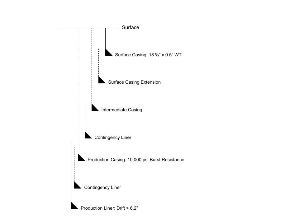
- Our surface casing has been determined as requiring a wall thickness of 0.5” - maybe this is a standard surface casing or structural load resistance dictates its design.
- Our Completions Engineering friends have informed us that they require a drift of at least 6.2” to fun their lower completion jewelry.
- The Production Technologist has informed us that the production casing must be good for 10,000 psi burst pressure - this is meant as just a simple scenario so we won’t go into what this requirement actually means.
- There’s a subsurface hazard below our surface casing that we wish to isolate with a surface casing extension.
- Beneath the intermediate casing, offset wells have sometimes encountered a loss zone across which we may need to deploy a contingency drilling liner.
- The target reservoir is beneath our produced main reservoir, which is heavily depleted. We’re not certain that we can make it to the well TD without a drilling liner.
A nice simple scenario to try out a few things. The first observation is that, given our connections data, the root of our paths is fixed - there’s only one connection that satisfies the wall thickness requirement. Similarly, we can discard any vertices in our graph that have an inner diameter drift of 6.2” or less. Another observations is that our design necessitates 7 casing strings, so we’re only interested in paths of length 7 or more.
Graph pruning
One of the nice things with graph-tool is the ability to filter the vertices or edges in the graph to create a view of the graph with only the vertices or edges that we’re interested in. We’ll now create a function that will filter out surface casings and any casing where the inner diameter or drift is less than the minimum specified by our Completion Engineers.
def set_vertex_filter(
    graph,
    surface_casing_size=18.625,
    surface_casing_wall_thickness=0.5,
    production_envelope_id_min=6.2
):
    # first let's filter out all vertices that are 18 5/8" except for the
    # one with the wall thickness of 0.5" that we desire
    filter_surface_casing = np.invert(np.all((
        graph.vp['size'].a >= surface_casing_size,
        graph.vp['pipe_body_wall_thickness'].a != surface_casing_wall_thickness
    ), axis=0))

    # we can also filter out anything that has an internal drift diameter of
    # 6.2" or smaller
    filter_leaves = np.invert(np.any((
        graph.vp['pipe_body_drift'].a <= production_envelope_id_min,
        graph.vp['pipe_body_inside_diameter'].a <= production_envelope_id_min,
        graph.vp['connection_inside_diameter'].a <= production_envelope_id_min
    ), axis=0))

    # create a boolean mask that we can apply to our graph
    graph_filter = np.all((
        filter_surface_casing,
        filter_leaves
    ), axis=0)

    # create a PropertyMap to store our mask/filter and assign our array to it
    graph.vp['vertices_filter'] = graph.new_vertex_property('bool')
    graph.vp['vertices_filter'].a = graph_filter

    # apply the filter to the graph
    graph.set_vertex_filter(graph.vp['vertices_filter'])

    # return the filtered graph
    return graph
Source and targets
Next we need to define our source and target nodes between which we want to find our paths. We’ll call them roots and leaves again and write a function for our specific scenario:
def get_roots_and_leaves(graph, surface_casing_size=18.625):
    roots = np.where(np.all((
        graph.vp['vertices_filter'].a,
        graph.vp['size'].a == surface_casing_size
    ), axis=0))[0]

    leaves = graph.get_vertices()[np.where(
        graph.get_out_degrees(graph.get_vertices()) == 0
    )[0]]

    return roots, leaves
Preliminary results
Let’s go ahead and see how we’re doing. We’ll write our main function that will run through all the functions we’ve created and return how many permutations we have and a few examples.
def main():
    # this runs the code from part 1 (make sure it's in your working directory)
    # and assigns the data to the variable catalogue
    catalogue = import_from_tenaris_catalogue.main()

    # initiate our graph and ray
    graph = make_graph(catalogue)
    ray.init()

    # add the casing connections from our catalogue to the network graph
    for product, data in catalogue.items():
        graph = add_vertices(
            graph,
            manufacturer='Tenaris',
            type='casing_connection',
            type_name=product,
            tags=data.get('headers'),
            data=data.get('data')
        )

    # determine which connections fit through which and add the appropriate
    # edges to the graph.
    graph = add_connection_edges(graph)

    graph = set_vertex_filter(graph)

    # place a copy of the graph in shared memory
    graph_remote = ray.put(graph)

    # # determine roots and leaves
    roots, leaves = get_roots_and_leaves(graph)


    # generate pairs of source and target nodes/vertices
    # we do this primarily to maximise utility of multiprocessing, to minimise
    # processor idling
    input = np.array(
        [data for data in map(np.ravel, np.meshgrid(roots, leaves))]
    ).T

    # loop through inputs and append paths to a list, using ray
    paths = ray.get([
        get_paths.remote(graph, s, t)
        for s, t in input
    ])

    # we end up with a list of lists which we need to flatten to a simple list
    paths = [item for sublist in paths for item in sublist]

    # we're only interested in paths of 7 or more
    paths_filtered_number_of_strings = [p for p in paths if len(p) >= 7]

    # we only want paths where the production casing (which is the 3rd string
    # from the end) has a maximum burst pressure larger than the 10,000 psi
    # requirement from our Production Technologist
    paths_filtered_production_casing_burst = [
        p for p in paths_filtered_number_of_strings
        if graph.vp['pipe_burst_pressure_max'].a[p[-3]] > 10000
    ]

    first_five = [
        [
            f"{graph.vp['size'][p]} in - {graph.vp['nominal_weight'][p]} ppf"
            for p in path
        ] for path in paths_filtered_number_of_strings[:5]
    ]

    print(
        f"Number of casing design permutations: "
        f"{len(paths_filtered_number_of_strings):,}"
    )
    print("First five permutations (size - nominal weight):")
    for path in first_five:
        print(path)

    return graph
To run the code we’ll add the following at the bottom of our script:
if __name__ == '__main__':
    graph = main()

    print("Done")
When we run the code, we see that we’ve significantly constrained the number of permutations down from millions to 3,796. A good reduction, but this is still far too many options to reasonably consider and from the first few results we can see there’s some quite unusual concepts that would require some none-standard equipment or cross-overs, so let’s see if we can filter these results a bit more by making a few more constraints.
['18.625 in - 100.0 ppf', '17.0 in - 77.5 ppf', '15.0 in - 77.5 ppf', '13.375 in - 54.5 ppf', '10.75 in - 40.5 ppf', '8.625 in - 32.0 ppf', '7.0 in - 20.0 ppf']
['18.625 in - 100.0 ppf', '17.0 in - 77.5 ppf', '15.0 in - 77.5 ppf', '13.375 in - 54.5 ppf', '10.75 in - 40.5 ppf', '8.625 in - 36.0 ppf', '7.0 in - 20.0 ppf']
['18.625 in - 100.0 ppf', '17.0 in - 77.5 ppf', '15.0 in - 77.5 ppf', '13.375 in - 54.5 ppf', '10.75 in - 40.5 ppf', '8.625 in - 40.0 ppf', '7.0 in - 20.0 ppf']
['18.625 in - 100.0 ppf', '17.0 in - 77.5 ppf', '15.0 in - 77.5 ppf', '13.375 in - 54.5 ppf', '10.75 in - 40.5 ppf', '8.625 in - 44.0 ppf', '7.0 in - 20.0 ppf']
['18.625 in - 100.0 ppf', '17.0 in - 77.5 ppf', '15.0 in - 77.5 ppf', '13.375 in - 54.5 ppf', '10.75 in - 40.5 ppf', '9.625 in - 36.0 ppf', '7.0 in - 20.0 ppf']
Refining the results
Let’s make a couple more constraints:
- We want to use a standard casing hanger in the first position, so let’s only consider casings in the third position that are smaller than 14” on their largest diameter.
- Similarly, our second position requires a casing smaller than 10”.
- We wish to maximize wall thickness for our production liner to maximize the well life in a potentially corrosive and abrasive environment.
- We want to trial a 16” expandable liner hanger.
Let’s apply a filter for item 1 in the list above (remember in Python that indexing starts at 0):
paths_filtered_first_position = [
        p for p in paths_filtered_number_of_strings
        if max(
            graph.vp['box_outside_diameter'].a[p[2]],
            graph.vp['coupling_outside_diameter'].a[p[2]]
        ) < 14.0
    ]
When we run this then we see that the length of the results is 0. Well that’s insightful since it means that we’re being too optimistic with our casing design objectives! What’s different now though it that we can demonstrate to our decision makers that we have literally tried every permutation to deliver the required functionality with the equipment that we have considered and it is not possible without relaxing our design constraints.
Take Two
Let’s remove that surface casing extension and leave that strategy to our deep water friends with their big bore wells.
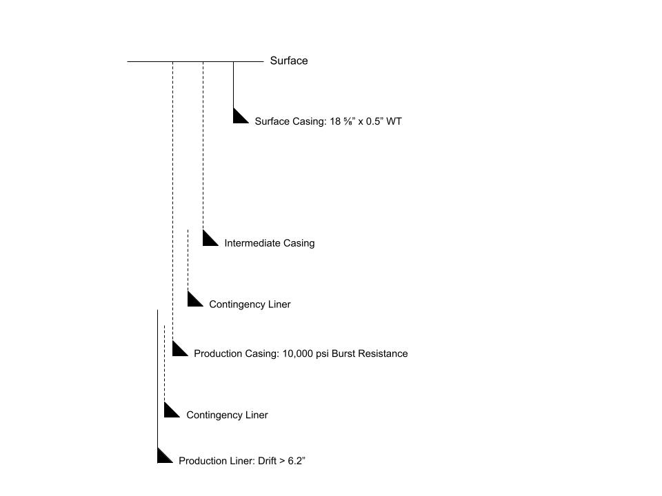
We’ll need to update our filter to reflect that we’re now looking for 6 casing strings rather than 7:
paths_filtered_number_of_strings = [p for p in paths if len(p) == 6]
If we rerun the code we find, again, that although we have options for a 6 string design, none of them satisfy our first position casing hanger constraint - that requirement for a production liner drift more than 6.2” is eating up our contingency options!
Probably at this point we might start looking at a 14” intermediate casing, but unfortunately with the casing connections that we’ve selected, this is not an option. An alternative might also be to consider some Solid Expandable Tubular (SET) drilling liner options, but again, these are not included in our data. So we’re forced to drop another contingency liner.
Take Three
We’ll aim to remove the intermediate casing contingency, resulting now in a 5 string design.
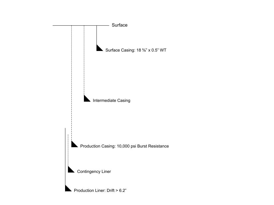
Updating our script:
paths_filtered_number_of_strings = [p for p in paths if len(p) == 6]
We find that we now have 2,592 concepts with 5 strings and the first hanger position occupied with a casing smaller than 14”. Let’s move onto refinement number 2, with the second hanger position occupied with a casing smaller than 10”.
We need to create another filter… we can just modify the previous filter for this:
paths_filtered_second_position = [
        p for p in paths_filtered_first_position
        if max(
            graph.vp['box_outside_diameter'].a[p[2]],
            graph.vp['coupling_outside_diameter'].a[p[2]]
        ) < 10
    ]
If we run this filter the result is… 0. This means, if we want that production casing contingency, then we need to run a larger diameter production casing but again, the difference now is that we have evidence to support this design change as we can state that given our environment, we have considered all of the available options.
So let’s now relax that second hanger position constraint to 11”:
paths_filtered_second_position = [
        p for p in paths_filtered_first_position
        if max(
            graph.vp['box_outside_diameter'].a[p[2]],
            graph.vp['coupling_outside_diameter'].a[p[2]]
        ) < 11
    ]
Excellent, we’re not down to just 220 casing design concepts. Let’s keep going with refinement number 3 where we select the maximum wall thickness we can for the production liner by using another filter:
paths_filtered_production_casing_wt_max = [
        p for i, p in enumerate(paths_filtered_second_position)
        if i in np.where(
            graph.vp['pipe_body_wall_thickness'].a == max([
                graph.vp['pipe_body_wall_thickness'].a[p[-1]]
                for p in paths_filtered_second_position
            ])
        )[0]
    ]
Almost there… we’re down to only 8 remaining casing design concepts.
Returning to our list, we find that refinement number 4 is now redundant since we made a decision not to run a contingency surface casing extension. So let’s think of something else - since we’re down to a single drilling liner contingency design, how about we minimize risk by selecting the design that offers us the maximum clearance between casing couplings, to potentially reduce sway and surge pressures and to improve the Probability of Success (POS) during our casing cementations?
We can write a quick little helper function for this and then call it for each of our paths and finally use these results to find our preferred design:
def get_clearance(graph, path):
        upper = path[:-1]
        lower = path[1:]

        clearance = sum([
            graph.ep['clearance'].a[graph.edge_index[graph.edge(u, l)]]
            for u, l in zip(upper, lower)
        ])

        return clearance

clearance = [
    get_clearance(graph, p)
    for p in paths_filtered_production_casing_wt_max

selected_concept = paths_filtered_production_casing_wt_max[
        np.argmax(clearance)
    ]
]
Below is a chart displaying our results: the nodes are the connections and the edges represent the feasible paths from our source 18 5/8” connection to our target connection(s) with at least 6.2” inner diameter (interesting how this resolved to a single target connection). The red path is the one with the maximum total clearance that we’ve defined as being our preferred path.
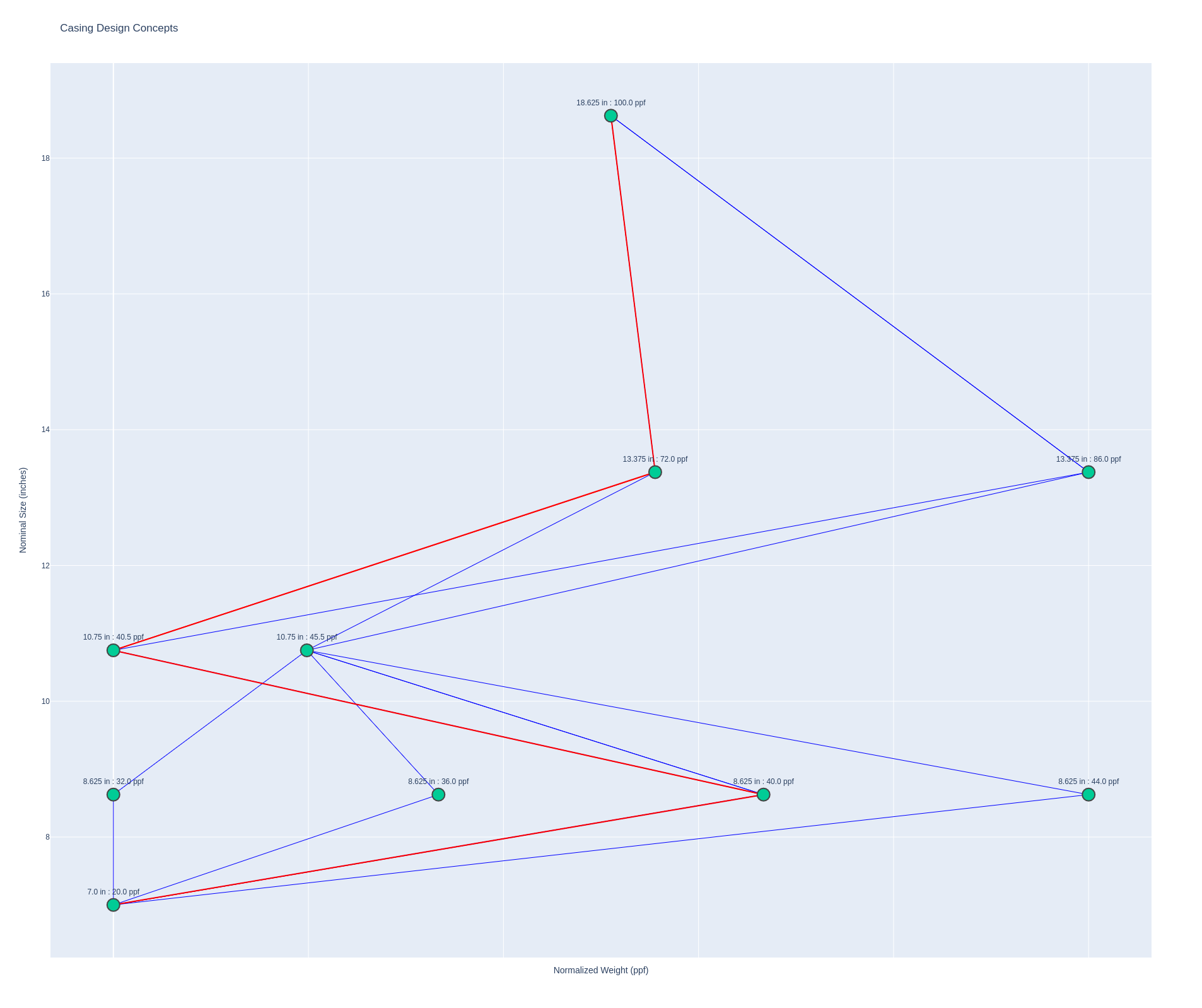
Congratulations, by constraining the option space and applying some filtering you’ve managed to collapse the casing design possibilities down from millions to one! Imagine if we could add not only additional casing connections, but well equipment like wellheads and their hangers, liner hangers, cross-overs and completion equipment. We’d then be able to create a method or workflow that would lead to determining a standardized well design architecture, one that’s repeatable and that demonstrably considers all permutations within a given given option space.
If only the equipment specifications were accessible.
Feel free to download the code, which included the function for generating the above chart.