Connection Conundrums - Part 3
In part 2 we took our imported catalogue data and used it to populate a network graph, linking casing connection nodes/vertices together with edges between casing connections that we’re interested in running together.
In this post, we’ll take a look at some functions for interrogating our network graph to provide us with casing design options.
Getting Started
First let’s import our libraries, including the script we wrote in the previous post (so make sure that the scripts from part 1 and part 2 are in your working directory).
import numpy as np
import networkx as nx
import create_casing_connections_graph # our code from part 2
We can now generate our graph object with the following line:
graph = create_casing_connections_graph.main()
Roots and leaves
So let’s answer the original question from part 1. To do this, we’re going to assume that we’re interested in only using these Tenaris Wedge 521 connections and that our surface casing size is 18 5/8”. We need a function that will identify all our root nodes/vertices (i.e. our 18 5/8” surface casing connections) and find all the paths to all the leaf nodes/vertices (which might be the completion tubing connection or the production liner connection).
A bit of background on graphs: the in_degree is the number of edges that lead into a node/vertex, while the out_degree is the number of edges that lead out of a node/vertex. A root has no edges leading into it and a leaf has no edges leading out of it. Think of a tree, with a root, branches and leaves.
The simplest way to get our roots (there can be more than one) and leaves is to loop though the nodes in the graph.
def get_roots_and_leaves(graph):
    # initiate our lists
    roots = []
    leaves = []
    # loop through our nodes to discover our start and end nodes
    for node in graph.nodes :
        if all((
            graph.in_degree(node) == 0, # it's a root
            graph.nodes[node]['size'] == 18+5/8
        )):
            roots.append(node)
        if graph.out_degree(node) == 0 : # it's a leaf
            leaves.append(node)

    return roots, leaves
Running the above function will return two lists, the first is the roots and the second the leaves. We can check these results with a quick bit of list comprehension:
>>> roots, leaves = get_roots_and_leaves(graph)
>>> [graph.nodes[r]['size'] for r in roots]
[18.625, 18.625, 18.625, 18.625, 18.625, 18.625, 18.625]
>>> [graph.nodes[l]['size'] for l in leaves]
[4.0, 4.0, 4.0, 4.5, 4.5, 4.5, 4.5, 4.5, 4.5, 7.625, 7.625, 7.625, 7.625, 7.625]
So we have 7 flavors of 18 5/8” casing connections for our roots and 14 leaves, ranging from 4” to 7 5/8”. We’ll use a bit of numpy to create our input array, which is all the permutations of roots and leaves (that’s 7 x 14 = 98)
input = np.array(
    [data for data in map(np.ravel, np.meshgrid(roots, leaves))]
).T
Paths
Now that we have our input with our source and target nodes/vertices (the surface casing and the production liner or tubing size), we can use these to determine all the paths in the graph between these pairs. Since there may be multiple paths for each pair of nodes/vertices, we’ll write a function to perform this:
def get_paths(graph, source, target):
    """
    Function for finding the paths between a source node and a target node in a graph, returning a list of nodes/vertices.
    """
    paths = [path for path in nx.all_simple_paths(graph, source, target)]
    return paths
We can then use our input array to feed our get_paths() function:
paths = [
    get_paths(graph, s, t)
    for s, t in input
]

# we end up with a list of lists which we need to flatter to a simple list
paths = [item for sublist in paths for item in sublist]
If you’ve got this far and you try running the above code, you’ll soon start to panic and think that you’ve done something wrong. You haven’t, it’s just that even with only 92 casing connections imported (and we’re not even considering different steel grades yet), there’s simply a huge number of permutations - which is why in part 1 I stated that Wells and Drilling Engineers are awesome because despite this huge number of options, they are able to quickly determine a suitable combination (albeit with a few subconscious tricks and an unfair degree of bias).
Let’s throw in some multiprocessing to speed things up, since I promised I’d tell you how many permutations there are. We’re going to use ray for this simply because it’s awesome and easier to use than Python’s built in multiprocessing.
Multiprocessing with ray
First install ray in our env with:
pip install -U ray
and then add it to our library imports with:
import ray
We’ll need to add a decorator to our get_paths() function to let ray know where to implement its magic (and you’ll see why I made this a function now… thinking ahead):
@ray.remote
def get_paths(graph, source, target):
    paths = [path for path in nx.all_simple_paths(graph, source, target)]
    return paths
We’re ready to write our main() function:
def main():
    # initialize ray
    ray.init()

    # generate our graph using code from previous post
    graph = create_casing_connections_graph.main()

    # place a copy of the graph in shared memory
    graph_remote = ray.put(graph)

    # determine roots and leaves
    roots, leaves = get_roots_and_leaves(graph)

    # generate pairs of source and target nodes/vertices
    input = np.array(
        [data for data in map(np.ravel, np.meshgrid(roots, leaves))]
    ).T

    # loop through inputs and append paths to a list, using ray
    paths = ray.get([
        get_paths.remote(graph_remote, s, t)
        for s, t in input
    ])

    # we end up with a list of lists which we need to flatten to a simple list
    paths = [item for sublist in paths for item in sublist]
    first_five = [
        [
            f"{graph.nodes[p]['size']} in - {graph.nodes[p]['nominal_weight']} ppf"
            for p in path
        ] for path in paths[:5]
    ]

    print(f"Number of casing design permutations: {len(paths):,}")
    print("First five permutations (size - nominal weight):")
    for path in first_five:
        print(path)
As usual, if we want to run this script, we need to add the following at the bottom:
if __name__ == '__main__':
    main()
Time to run it!
Results
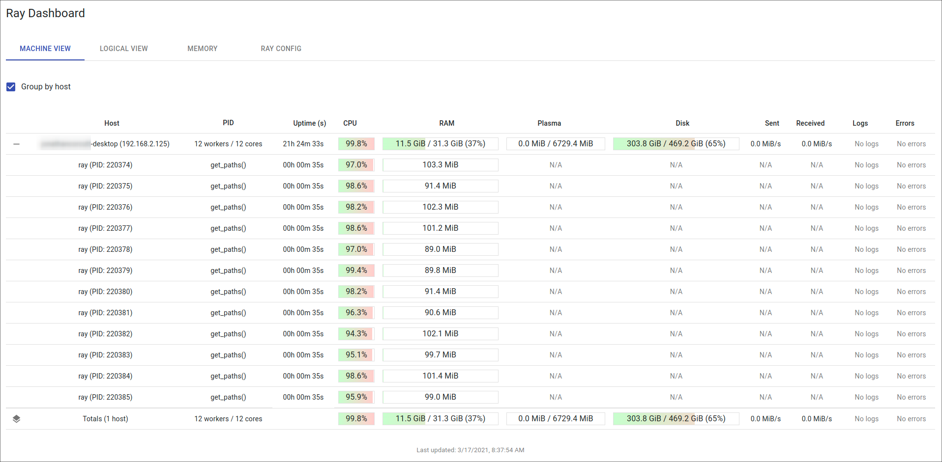
One of the nice features of ray is that it serves a dashboard which can be viewed via your web browser (you’ll be provided with a link with the local address and port that you can click on, the default is http://127.0.0.1:8265). By default, ray will utilize all of the available cores on your machine, which in my case is 12 as you can see from the screenshot below - it’s satisfying to know that your hurting your processor.
Setting my enthusiasm for ray aside, the answer to the ultimate question is not 42 as you might have expected, but rather:
5,080,320
Yep, from 92 connections we can generate this many permutations of casing design even with some constraints. As QAQC to verify that the results make sense, we’ve added a print loop to show the size and weight of the casing for the first five entries in our paths list:
['18.625 in - 87.5 ppf', '13.375 in - 54.5 ppf', '9.625 in - 36.0 ppf', '7.0 in - 20.0 ppf', '5.0 in - 13.0 ppf', '4.0 in - 9.5 ppf']
['18.625 in - 87.5 ppf', '13.375 in - 54.5 ppf', '9.625 in - 36.0 ppf', '7.0 in - 20.0 ppf', '5.0 in - 15.0 ppf', '4.0 in - 9.5 ppf']
['18.625 in - 87.5 ppf', '13.375 in - 54.5 ppf', '9.625 in - 36.0 ppf', '7.0 in - 20.0 ppf', '5.0 in - 18.0 ppf', '4.0 in - 9.5 ppf']
['18.625 in - 87.5 ppf', '13.375 in - 54.5 ppf', '9.625 in - 36.0 ppf', '7.0 in - 23.0 ppf', '5.0 in - 13.0 ppf', '4.0 in - 9.5 ppf']
['18.625 in - 87.5 ppf', '13.375 in - 54.5 ppf', '9.625 in - 36.0 ppf', '7.0 in - 23.0 ppf', '5.0 in - 15.0 ppf', '4.0 in - 9.5 ppf']
Can you spot the differences?
I think we’ve earned a coffee break after all that exertion - next post we’ll see if we can do some pre-processing to reduce our options space and limit the path search as clearly it’s not practical to calculate all the paths from the connections, especially if we want to start adding all casing connections to our catalogue.
Feel free to download the code.