Connection Conundrums - Part 2
In part 1 we imported some connections data from a pdf catalogue and we finished with a dictionary called catalogue in which we had a list of arrays, the index of which corresponded with the column headers in the template dictionary, which we combined together into a pandas DataFrame so that we could QAQC the data.
Permutations
There are 92 Wedge 521 connections in our newly created catalogue, ranging in size from 18 5/8” to 4” (the nominal diameter of the pipe body). How many different ways can we combine these connections?
Definitions
First, let’s be clear what we mean by combine. For me, a valid combination is when one connection on pipe can pass through another connection on pipe. That means that the largest outer diameter of smaller size connection and pipe must be less than the drift of the larger coupling and pipe.
That escalated quickly
So, for each coupling, we need to test it against every other coupling to see if it will “drift”. If there’s 92 connections, that means we have to make 92 x 91 = 8,372 checks to see which connection fits through what. Once we know what fits through what, we need to string together combinations of these pairs. There’s a nice bit of maths that can help us here called network theory.
Building relationships
Fortunately, there are a number of Python implementations of network graphs but for this exercise we’re going to use networkx, simply because it’s the simplest to install and easiest to work with. This comes at the cost of speed, but for the time being let’s not worry about that.
You’ll need to install networkx in your Python env with the following terminal command:
pip install networkx
Then we can start writing some code, importing our libraries (including the code we wrote last time - note that I made a couple of changes to the code from last time, so be sure to get the latest version):
import numpy as np
import networkx as nx
import import_from_tenaris_catalogue  # our code from part 1

# this runs the code from part 1 (make sure it's in your working directory)
# and assigns the data to the variable catalogue
catalogue = import_from_tenaris_catalogue.main()
Before we start, each node in our graph needs to have a unique identifier (UID) which we don’t currently have in our catalogue. So let’s quickly create a Counter class that we can use to generate UID.
class Counter:
    def __init__(self, start=0):
        """
        A simple counter class for storing a number that you want to increment
        by one.
        """
        self.counter = start

    def count(self):
        """
        Calling this method increments the counter by one and returns what was
        the current count.
        """
        self.counter += 1
        return self.counter - 1

    def current(self):
        """
        If you just want to know the current count, use this method.
        """
        return self.counter
This counter will run in the background and we can call it for a new UID each time we create a node for our graph and assign that UID to the new node.
To initiate a new graph, which we’ll call graph, we use the following code:
graph = nx.DiGraph()
Adding vertices (nodes)
We’ve now initiated an instance of a DiGraph class, the Di denoting that this is a directional graph, so the edges we’ll be adding will be one way (which will prevent looping when we start navigating the graph). It’s time start adding nodes, but since our connections have 17 attributes each that we want to add to the node, we’ll write a function for this.
def add_node(
    counter, graph, manufacturer, type, type_name, tags, data
):
    """
    Function for adding a node with attributes to a graph.

    Parameters
    ----------
    counter: Counter object
    graph: (Di)Graph object
    manufacturer: str
        The manufacturer of the item being added as a node.
    type: str
        The type of item being added as a node.
    type_name: str
        The (product) name of the item being added as a node.
    tags: list of str
        The attribute tags (headers) of the attributes of the item.
    data: list or array of floats
        The data for each of the attributes of the item.

    Returns
    -------
    graph: (Di)Graph object
        Returns the (Di)Graph object with the addition of a new node.
    """
    # we'll first create a dictionary with all the node attributes
    node = {
        'manufacturer': manufacturer,
        'type': type,
        'name': type_name
    }
    # loop through the tags and data
    for t, d in zip(tags, data):
        node[t] = d
    # get a UID and assign it
    uid = counter.count()
    node['uid'] = uid

    # overwrite the size - in case it didn't import properly from the pdf
    size = (
        node['pipe_body_inside_diameter']
        + 2 * node['pipe_body_wall_thickness']
    )
    # use the class method to add the node, unpacking the node dictionary
    # and naming the node with its UID
    graph.add_node(uid, **node)

    return graph
We’ll use the above function to add all our connections to the graph, but once all these nodes or vertices are added, we need to connect them together with edges to indicate which connections can pass through which.
Adding edges
We’ll use two functions for this, one for adding an edge and the other a helper function. First the helper function.
def check_connection_clearance(graph, node1, node2, cut_off=0.7):
    """
    Function for checking if one component will pass through another.

    Parameters
    ----------
    graph: (Di)Graph object
    node1: dict
        A dictionary of node attributes.
    node2: dict
        A dictionary of node attributes.
    cut_off: 0 < float < 1
        A ration of the nominal component size used as a filter, e.g. if set
        to 0.7, if node 1 has a size of 5, only a node with a size greater than
        3.5 will be considered.

    Returns
    -------
    graph: (Di)Graph object
        Graph with an edge added if node2 will drift node1, with a `clearance`
        attribute indicating the clearance between the critical outer diameter
        of node2 and the drift of node1.
    """
    try:
        node2_connection_od = node2['coupling_outside_diameter']
    except KeyError:
        node2_connection_od = node2['box_outside_diameter']
    clearance = min(
            node1['pipe_body_drift'],
            node1['connection_inside_diameter']
    ) - max(
        node2_connection_od,
        node2['pipe_body_inside_diameter']
        + 2 * node2['pipe_body_wall_thickness']
    )
    if all((
        clearance > 0,
        node2['size'] / node1['size'] > cut_off
    )):
        graph.add_edge(node1['id'], node2['id'], **{'clearance': clearance})

    return graph
This is essentially checking the largest outside diameter of the node2 component against the drift of the node1 component. However, you’ll see that there’s a filter added, the cut_off parameter - we could link all components that pass through each other in the network graph (e.g. a 4” connection will pass through an 18 5/8” connection), but this will make our decision space unnecessarily large - would we design a well where we run a 4” tubing directly inside an 18 5/8” surface casing? If we do want to consider these options, then we can set cut_off=0, but the default is set cut_off=0.7, which for example means that we’re looking for sizes larger than 13” to run inside our 18 5/8” surface casing.
Now we can write our edge function.
def add_connection_edges(graph, cut_off=0.7):
    """
    Function to add edges between connection components in a network graph.

    Parameters
    ----------
    graph: (Di)Graph object
    cut_off: 0 < float < 1
        A ration of the nominal component size used as a filter, e.g. if set
        to 0.7, if node 1 has a size of 5, only a node with a size greater than
        3.5 will be considered.

    Returns
    -------
    graph: (Di)Graph object
        Graph with edges added for connections that can drift through other
        connections.
    """
    for node_outer in graph.nodes:
        # check if the node is a casing connection
        if graph.nodes[node_outer]['type'] != 'casing_connection':
            continue
        for node_inner in graph.nodes:
            if graph.nodes[node_inner]['type'] != 'casing_connection':
                continue
            graph = check_connection_clearance(
                graph,
                graph.nodes[node_outer],
                graph.nodes[node_inner],
                cut_off
            )
    return graph
This is not a particularly efficient way to add our edges, but for the purposes of this exercise using a small dataset for illustration, then it will suffice. For larger datasets, filtering the nodes/vertices with numpy and multiprocessing with e.g. ray would get this done much faster.
Bringing it all together
Finally, we’ll write our main function to run the above and generate our
populated network graph.
def main():
    # this runs the code from part 1 (make sure it's in your working directory)
    # and assigns the data to the variable catalogue
    catalogue = import_from_tenaris_catalogue.main()

    # initiate our counter and graph
    counter = Counter()
    graph = make_graph(catalogue)

    # add the casing connections from our catalogue to the network graph
    for product, data in catalogue.items():
        for row in data['data']:
            graph = add_node(
                counter,
                graph,
                manufacturer='Tenaris',
                type='casing_connection',
                type_name=product,
                tags=data['headers'],
                data=row
            )

    # determine which connections fit through which and add the appropriate
    # edges to the graph.
    graph = add_connection_edges(graph)

    return graph
Results
To run the above script, we can add the following at the bottom of our .py file:
if __name__ == '__main__':
graph = main()
# as a QAQC step we can use matplotlib to draw the edges between connected
# casing connections
import matplotlib
import matplotlib.pyplot as plt
matplotlib.use("TKAgg") # Ubuntu sometimes needs some help
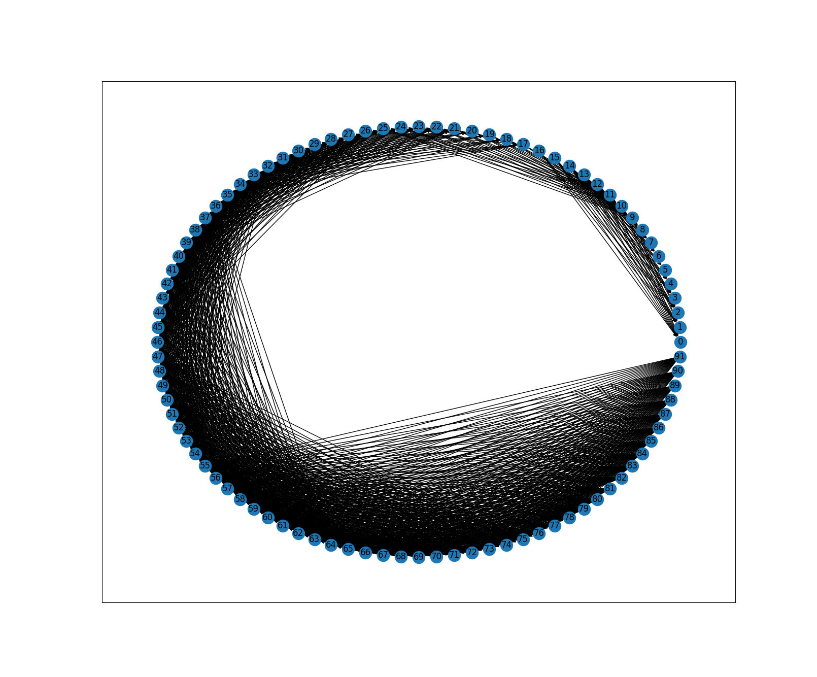
nx.draw_networkx(graph, pos=nx.circular_layout(graph))
plt.show()
print("Done")
You’ll see that we’re importing matplotlib here as a QAQC step to visually check that we have indeed imported the 92 connections from the catalogue and that we have successfully created edges between connections where one will drift through another.
 Congratulations, you’ve just created a network graph and populated it with some casing connections and linked together connections that will drift through other connections. In the next post we’ll see how we can list the different permutations of casing we can deploy in our well and how we can filter the data to provide us with choices for our specific environment.
Feel free to download the code.