Modified Tortuosity Index: Maximum Curvature and Survey Frequency

Summary

This post proposes a Maximum Curvature method for creating a well trajectory with a defined incremental Dog Leg Severity (DLS) and a more realistic tortuosity versus trajectories constructed with the Minimum Curvature method. The post further investigates the impact of survey station frequency on calculated Modified Tortuosity Index values and proposes a three step method to systematically and repeatably calculate a realistic tortuosity for sparse and dense surveys alike.

Disclaimer

The following method is experimental and has yet to be thoroughly tested - the work presented is that of an enthusiastic amateur, with no professional or otherwise affiliations. As such, please use with caution and do your own research and testing - the only request is that, in the spirit of open source you report back your own findings either via the comments below or via the welleng repository. The license is permissive - the only requirement is that you reference the source if you use the methods or code presented herein.

Background

A sparsely populated survey can have considerable geometric uncertainty which can overlooked and the MTI can be underestimated for a well path. Take the example illustrated in the figure below:

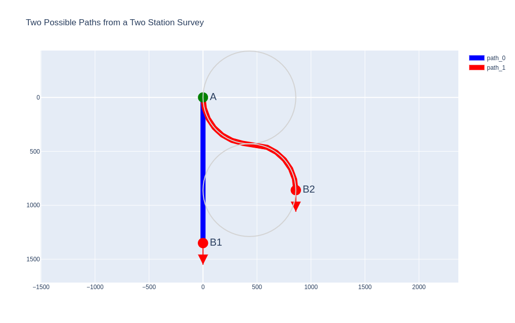Two possible paths for a two station survey. In this example, the radius of curvature for path_0 is equivalent to a 4 deg/30m DLS (reference the grey circles) and both path lengths are \(\pi \times radius\) meters. The well path unit vectors at B1 and B2 are equal and represented by the arrows.

Both paths (path_0 and path_1) have a common start point with identical positions, vectors (inclination and azimuth) and measured depths. Only a single survey station at the TD of the well is provided - it’s an MWD survey with a measured depth (MD), inclination and azimuth. The vector at position B1 is identical to the vector at position B2. Since there’s no description or data to define the path between these two points, path_0 and path_1 are both valid paths (although path_0 may be more likely) but clearly path_1 is significantly more tortuous. It’s also clear the impact that these paths have on the final location of the well, but that discussion is out of scope for this post.

Maximum Curvature Method

The minimum curvature method does precisely what it says - it fits a path between two survey stations with the minimum amount of curvature. What we need though is a method that consistently and repeatably fits a prescribed amount of additional curvature to a path between two points.

In previous posts we noted that the minimum curvature is determined across a plane that is defined by the cross product of the normal vector (between two subsequent survey stations) and the survey station vector, which means we can simplify our maximum curvature method by constraining it to the two dimensions of the curvature plane.

If you’ve ever had the opportunity to observe a Directional Driller steering a bent sub and motor assembly, you may have noticed that they typically perform the majority of steering (sliding) in the first section of the stand and then drill down the remainder of the stand in rotary mode. We can apply this same philosophy (and perhaps simulate a well path drilled with a bent sub and motor) by applying additional curvature (increased dogleg) to the first half of the path between two survey stations and allowing the curvature to correct itself for the second half of section (using minimum curvature from the midpoint to the end point of the section).

Let’s say we have two survey stations and using minimum curvature we calculate a Dog Leg Severity (DLS) of 2 deg/30m for a path to connect these points. To introduce some additional curvature to the section, we can add an additional 1 deg/30m DLS to the first half of the section and apply this curvature in the same plane, so 3 deg/30m with the same initial toolface setting. For the remainder of the section we now need to reduce the DLS so that we still end up with the same inclination and azimuth (vector) for the same interval length as described by the two survey stations.

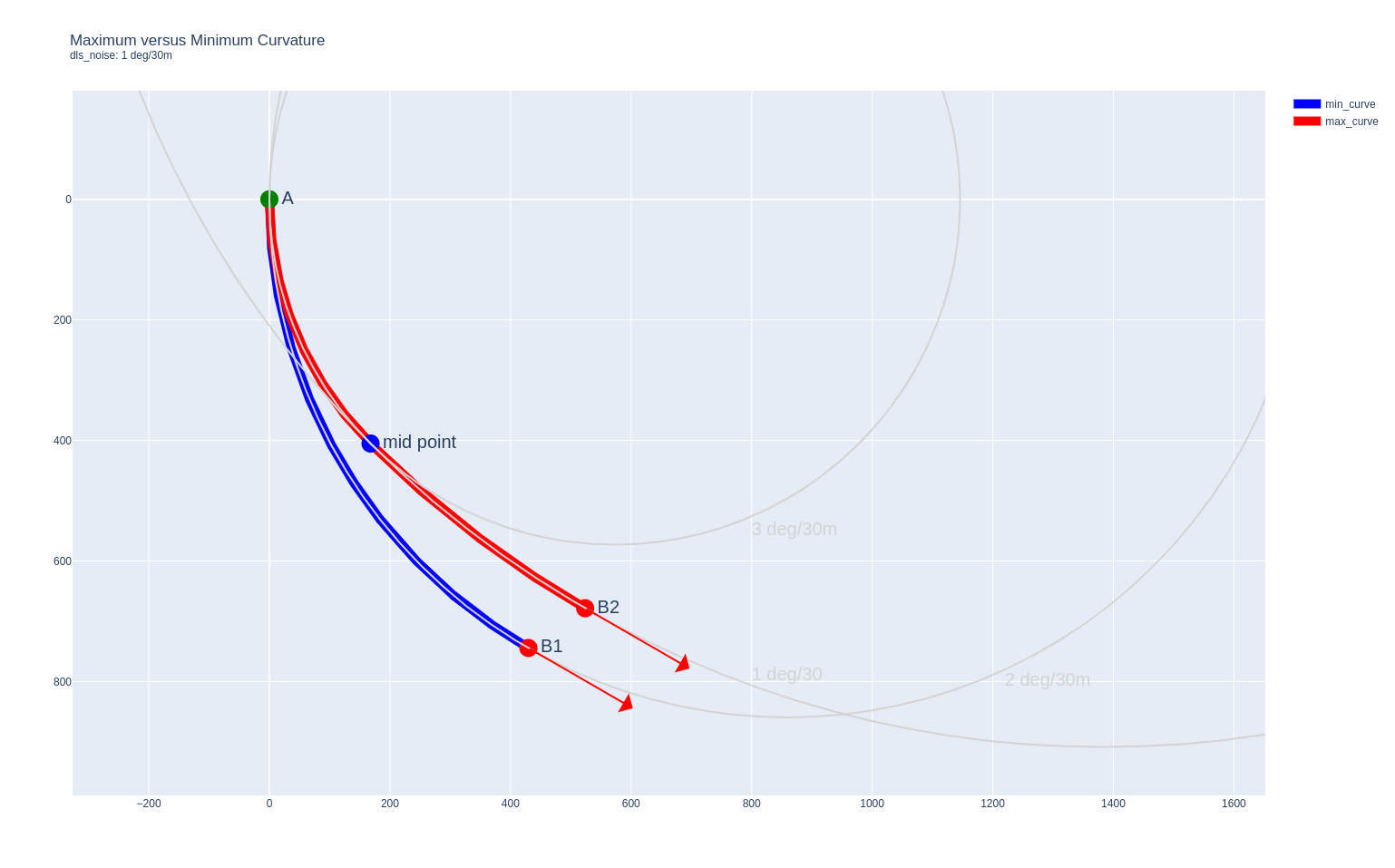Connecting survey stations A and B with the maximum (red) versus the minimum (blue) curvature methods, using an incremental 1 deg/30m Dog Leg Severity (DLS) for the first half of the maximum curvature path.

Here’s some code describing the Maximum Curvature Method:

import numpy as np
import welleng as we

def maximum_curvature(survey, dls_noise=1.0):
    """
    Create a well trajectory using the Maximum Curvature method.

    Parameters
    ----------
    survey: welleng.Survey.survey object
    dls_noise: float
        The additional Dog Leg Severity (DLS) in deg/30m used to calculate the
        curvature for the initial section of the survey interval.
    
    Returns
    -------
    survey_new: welleng.survey.Survey object
        A revised survey object calculated using the Minimum Curvature method
        with updated survey positions and additional mid-point stations.
    """

    # Iterate through survey station pairs.
    for i, ((md2, vec2, dls), (md1, vec1, survey1)) in enumerate(zip(
        zip(survey.md[1:], survey.vec_nev[1:], survey.dls[1:]),
        zip(survey.md[:-1], survey.vec_nev[:-1], survey.survey_rad[:-1])
    )):
        # add the first survey station to the new survey
        if i == 0:
            _survey_new = [
                [md1, *np.degrees(we.utils.get_angles(vec1, nev=True))[0]]
            ]
        
        # Calculate the vector of the normal plane between of two stations or
        # set to NaN if the vectors are parallel.
        vec_normal = np.cross(vec1, vec2)
        vec_normal = np.nan if np.all(vec_normal==0.0) else vec_normal

        # Calculate the (minimum) curvature radius.
        vec_radius = (
            np.inf if np.all(np.isnan(vec_normal))
            else np.cross(vec_normal, vec1)
        )

        # Calculate the initial toolface - this is used to determine the
        # rotation angle which is used for a transform later. The welleng
        # library has a function for converting from the NEV to HLA domain.
        if np.all(vec_radius == np.inf):
            toolface1 = 0.0
        else:
            _, toolface1 = we.utils.get_angles(we.utils.NEV_to_HLA(
                survey1, vec_radius, cov=False
            ), nev=True).T

        # Calculate the new initial DLS and convert to a curvature radius.
        dls_effective = dls + dls_noise
        radius = we.utils.radius_from_dls(dls)
        radius_effective = we.utils.radius_from_dls(dls_effective)

        # Manage where the path is straight.
        if dls == 0:
            dogleg1 = ((md2 - md1) / radius_effective) / 2
        else:
            dogleg1 = ((md2 - md1) / radius_effective) / 2
        
        # For simplicity, limit the maximum dogleg to 90 degrees - this will
        # be fine for 99% of the time and where it isn't there's likely so
        # more pressing issues with the trajectory.
        if dogleg1 > np.pi:
            dogleg1 = np.pi
            radius_effective = (md2 - md1) * 4 / (2 * np.pi)

        # Use the welleng function to create the first half of the well path
        # as a simple arc and rotate and transform to the survey station.
        arc1 = we.utils.get_arc(dogleg1, radius_effective, toolface1, vec=vec1)

        # Add the new point (the end of the newly created arc) to the new
        # survey.
        _survey_new.append([
            _survey_new[-1][0] + arc1[-1],
            *np.degrees(we.utils.get_angles(arc1[1], nev=True))[0]
        ])

        # The survey station at the end of the section is simply the second
        # survey station, so append this to the list. When the new survey is
        # calculated using minimum curvature, the required degree of DLS will
        # be calculated to return the path to the survey station.
        _survey_new.append([
            md2, *np.degrees(we.utils.get_angles(vec2, nev=True))[0]
        ])
    
    # Transform array to Series of md, inc and azi.
    md, inc, azi = np.vstack(_survey_new).T

    # Update the new survey header as the new azimuth reference is 'grid'.
    sh = survey.header
    sh.azi_reference = 'grid'

    # Create a new Survey instance.
    survey_new = we.survey.Survey(
        md=md,
        inc=inc,
        azi=azi,
        header=sh,
        start_xyz=survey.start_xyz,  # transforms to the original survey start
        start_nev=survey.start_nev  # transforms to the original survey start
    )
    
    return survey_new

We now have a function for determining mid-points between MWD survey station pairs, adding a defined increment of DLS for the first sub-interval and using the Minimum Curvature method to calculate the second half of the path back to the final survey station.

Note that the function uses the welleng library as a dependency, but can be easily modified to process raw survey data. Also, a vectorized (quicker) version of this code has been added to welleng version 0.4.13 as a Survey.maximum_curvature() method and the Survey.modified_tortuosity_index() method has been updated to apply by default the three step process and default values discussed in this post.

Applying Maximum Curvature to a Sparse Survey

Let’s apply the Maximum Curvature method to a fictitious sparse survey. For consistency we’ll again use the ISCWSA Example 2 trajectory which is generated with the following function:

import numpy as np
import welleng as we


def get_iscwsa_example_2():
    # ISCWSA No. 2
    # survey header data
    header = we.survey.SurveyHeader(
        name="ISCWSA No. 2: Gulf of Mexico fish-hook well",
        latitude=28,
        longitude=-90,
        G=9.80665,
        b_total=48_000,
        dip=58,
        declination=2,
        vertical_section_azimuth=21,
        azi_reference='true'
    )

    # generate survey array - these are in feet
    md, inc, azi = np.array([
        [0.0, 0.0, 0.0],
        [2000.0, 0.0, 0.0],
        [3600.0, 32.0, 2.0],
        [5000.0, 32.0, 2.0],
        [5525.54, 32.0, 32.0],
        [6051.08, 32.0, 62.0],
        [6576.62, 32.0, 92.0],
        [7102.16, 32.0, 122.0],
        [9398.5, 60.0, 220.0],
        [12500.0, 60.0, 220.0]
    ]).T

    # initiate Survey instance
    survey = we.survey.Survey(
        md * 0.3048,  # convert to meters
        inc, azi,
        header=header
    )
    return survey

Generating the survey data and calculating the Maximum Curvature trajectory can now be done using the functions defined above, setting dls_noise=1.0 deg/30m:

survey = get_iscwsa_example_2()

survey_maxc = maximum_curvature(survey, dls_noise=1.0)

Let’s visually compare these two trajectories, using the welleng Survey convenience method figure() to generate the plot data:

# Generate the figure data - interpolation is done to generate smooth plots
# with enough data points to appear as a continuous curvature.
fig = survey_maxc.interpolate_survey(step=30).figure()
fig.data[1].visible = False
fig.data[0].name = 'survey_max_curvature'

_fig = survey.interpolate_survey(step=30).figure()
_fig.data[1].visible = False
_fig.data[0].name = 'survey_min_curvature'

# Combine the figure data into a single figure
for i, trace in enumerate(_fig.data):
    fig.add_trace(trace)

# Change the colors of the Minimum Curvature traces
fig.data[5]['marker']['color'] = 'black'
fig.data[3]['line']['color'] = 'black'

fig.show()

This generates the following plot:

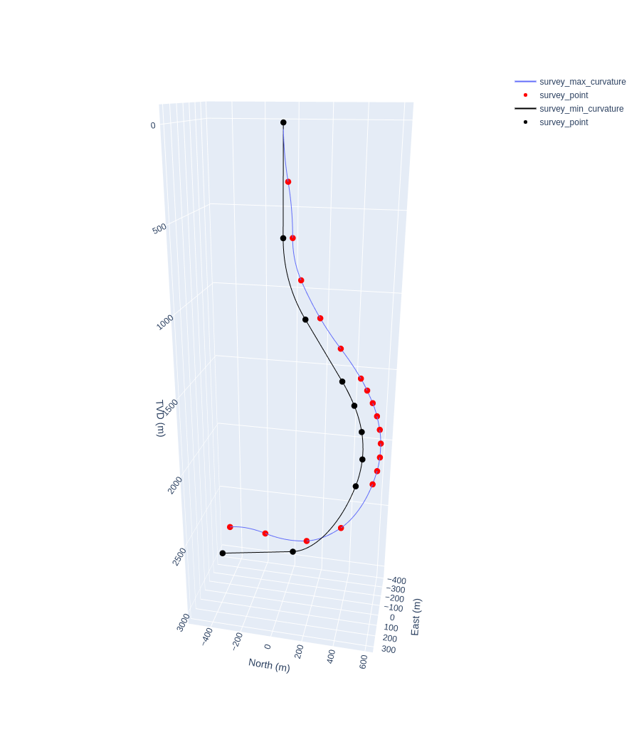Comparison of well trajectories generated using Maximum Curvature versus Minimum Curvature methods from identical survey station data (md, inc, azi).

Clearly, geometric uncertainty in sparse surveys can result in significant position uncertainty, something I believe is overlooked in the current survey error models like the current ISCWSA Rev 5 model. If we take a closer look at the two well trajectories we can see that the Maximum Curvature trajectory (blue with red survey stations) has twice as many points as the addition of mid-points is required - from a processing perspective it will be important to flag and differentiate these additional points as having been calculated rather than being true survey stations.

When this plot was presented on LinkedIn there were a number of comments about the Maximum Curvature profile not being realistic or useful, that a competent Directional Driller would never drill such a trajectory and that we some context (the Directional Driller’s notes/records which the operator never gets to see) this extreme representation can be neglected and a more realistic interpretation determined. We’ll try and address this feedback below.

Incorporating Maximum Curvature into the Modified Tortuosity Index Method

Recall that the point of this series of posts is to proposed an updated method for calculating Tortuosity Index for a well trajectory and that in the process of validating this method we uncovered that the tortuosity of a well is dependent on the frequency of survey stations - real surveys with less stations will appear to be less tortuous than identical surveys with more survey stations.

Using the Maximum Curvature method, we should be able to penalize sparse surveys to give a more realistic indication of actual tortuosity. Let’s test this hypothesis.

Using welleng we can simply calculate the Modified Tortuosity Index (MTI) for the two trajectories created above:

mti_survey = survey.modified_tortuosity_index()
mti_survey_maxc = survey_maxc.modified_tortuosity_index()

If we now compare the MTI at the well TD for the two trajectories we see the following:

Well	Modified Tortuosity Index
Minimum Curvature	0.671
Maximum Curvature	0.782

This of course is not an unexpected result, but confirms that the method is working - using the Maximum Curvature method to fit a trajectory through a survey does result in a more tortuous well path. Also note that the test survey we’re using (ISCWSA Example 2) could be considered a design trajectory - if the MTI method were being used to define a Key Performance Indicator between an operator and a Directional Drilling service company, agreeing on a dls_noise parameter and using the Maximum Curvature method to define a target MTI value seems like a reasonable proposal.

However, there’s more to explore here.

Effect of Interval Length on MTI using Maximum Curvature

Let’s address that LinkedIn feedback.

If we assume that generally/historically survey station frequency is defined by a stand length (taken when making a connection) then it’s not unreasonable to define this section length when calculating the Maximum Curvature trajectory.

Using the welleng Survey.interpolate_survey() method, we can interpolate the survey to provide a calculated survey station at least every 30 meters:

survey.interpolate_survey(step=30)

This will return a new survey which includes interpolated survey stations every 30 meters (defined by the step=30 parameter). What happens if we use this interpolated survey as input into the maximum_curvature() function and calculate the MTI from this trajectory?

survey_maxc = maximum_curvature(survey.interpolate_survey(step=30), dls_noise=1.0)

Let’s plot this new trajectory against the original one:

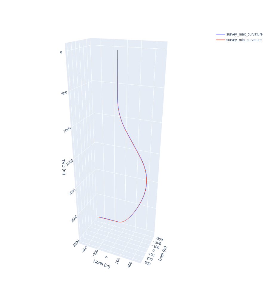Comparison of well trajectories generated using Maximum Curvature versus Minimum Curvature methods from identical survey station data (md, inc, azi) where the original survey has been interpolated to generate a calculated survey station every 30 meters.

That’s interesting (although maybe not completely unexpected) - now the two surveys lie almost on top of each other. Lets zoom into the last few hundred meters and see what the difference in final locaion looks like:

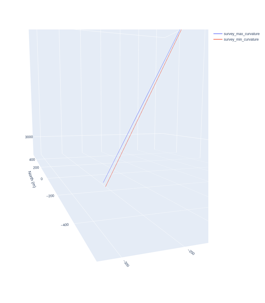Above figure, zoomed into the final few hundred meters to the well TD to indicate the well path separation.

Clearly using the interpolated trajectory has had a large effect on the position uncertainty, reducing it down to just a few meters at the well TD - again, perhaps not an unexpected result. Let’s calculate the MTI and see what impact it’s had on this:

Well	Modified Tortuosity Index
Minimum Curvature	0.671
Maximum Curvature	0.782
Maximum Curvature with 30m interpolation	0.847

Well that is interesting - by interpolating the original survey every 30 meters and then calculating a Maximum Curvature trajectory we not only have a well path that better matches the original survey, but it also increases the MTI.

So what’s the optimal step length? Using some multiprocessing magic we can quickly generate some MTI data for a range of step values:

import ray
ray.init()

@ray.remote
def get_mti(survey, step, dls_noise):
    mti = maximum_curvature(
        survey.interpolate_survey(step=step), dls_noise=1.0
    ).modified_tortuosity_index()[-1]

    return mti


mti = ray.get([
    get_mti.remote(survey, step, dls_noise=1.0)
    for step in np.linspace(0.1, 1000.0, 1000)
])
ray.shutdown()

And now plot the results:

import plotly.graph_objects as go

fig = go.Figure()
fig.add_trace(
    go.Scatter(
        x=np.linspace(0.1, 1000.0, 1000),
        y=mti
    )
)
fig.update_layout(
    title=(
        f'Modified Tortuousity Index Versus Interpolated Step Length'
        f'<br><sup>Using Maximum Curvature method with dls_noise: 1 deg/30m</sup>'
    ),
    xaxis=dict(
        type='log',
        showgrid=True,
        title='Interpolation Step (meters)'
    ),
    yaxis=dict(
        title='Modified Tortuosity Index'
    )
)
fig.add_vline(
    x=30, line_width=3, line_color='red'
)
fig.add_vline(
    x=1, line_width=3, line_color='green'
)

fig.show()

This will generate the following plot:

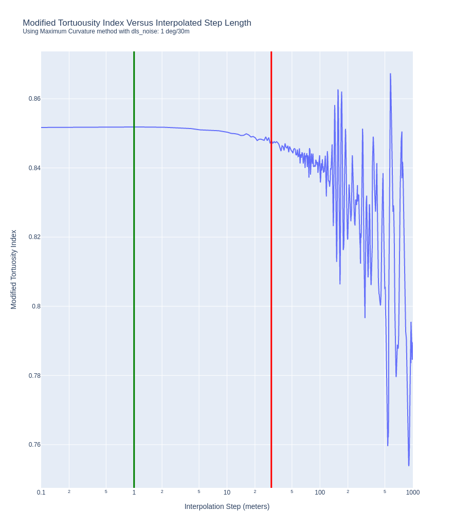The effect of interpolated step length on the Modified Tortuosity Index value.

From the plot and for the example well, the MTI value is noisy with step values above 100 meters and looks to trend towards an asymptote with the step value at around 1 meter (the green vertical line). A step length of 30 meters (the red vertical line) looks okay in terms of noise but with a large error relative to the asymptotic MTI value.

From this chart, a default interpolation step value of 1 looks to give an MTI result that is reasonably close to the asymptotic MTI value.

Conclusions

By using an interpolated directional survey with a step length of 1.0 meter and using the Maximum Curvature method with a suggested default dls_noise parameter of 1.0 deg/30m to generate the well trajectory in cartesian space, the Modified Tortuosity Index (MTI) can be used to consistently gauge the realistic tortuosity of a well path regardless of the frequency of survey stations.

This three step method is further proposed for determining a Key Performance Indicator (KPI) for a designed well path - the performance of the Directional Drilling service provider can be assessed by comparing the design MTI value versus the as drilled derived MTI value.

Further testing and refinement is required and recommended before applying this method.

As usual, please feel free to leave any comments or feedback.