An Example of using welleng's Torque and Drag module
 Applying some torque
In version 0.4.9 of the welleng library, the torque_drag module has been rewritten to reproduce the method described Torque and Drag in Directional Wells–Prediction and Measurement by C.A. Johancsik et al. This post runs through how to replicated one of the examples in the paper using welleng.
Getting Started
Start by installing welleng in your Python environment - I recommend making a fresh conda environment using the excellent conda cheat sheet to guide you:
>>> conda create --name welleng python==3.7
>>> conda activate welleng
>>> pip install welleng[easy]
Now start up your favorite development environment and create a new .py file - my preference is Visual Studio Code.
Create a Trajectory
The reference paper gives three example wells, but only the results for one of them, so we’ll recreate that one, example 3.
Import the welleng library and to save some typing we’ll set a local variable pointing at the new units module.
import welleng as we

ureg = we.units.ureg
The paper lists some control points for the three example wells and we’ll use the ones for example 3 to define some control nodes.
node0 = we.node.Node(pos=[0, 0, 0], md=0, inc=0, azi=0)
node1 = we.node.Node(md=731.5, inc=0, azi=0)
node2 = we.node.Node(md=1280, inc=44, azi=0)
node3 = we.node.Node(md=3718, inc=44, azi=0)
The first node is the starting point with the cartesian coordinates [0, 0, 0], starting measured depth of 0 meters and inclination and azimuth both set to 0 degrees.
The well is vertical down to the second node at 731.5 meters where it kicks-off towards the third node’s inclination of 44 degrees. The well holds this inclination and azimuth to the section TD with measured depth of 3718 meters at the final node.
We’ll use welleng’s Connector class to make sections of trajectory connecting up these nodes, appending these to a list that we can use to create a Survey with 30 meter intervals interpolated between the control nodes.
# create an empty list
connectors = []

# append the first connector from the first to the second node
connectors.append(
    we.connector.Connector(node0, node1)
)

# us the newly created node in the connector list and connect it to the third node
connectors.append(
    we.connector.Connector(connectors[-1].node_end, node2, dls_design=2)
)

# similarly connector the current last node in the list to the final node
connectors.append(
    we.connector.Connector(connectors[-1].node_end, node3, dls_design=4)
)

# use the list of connectors as input to create a Survey instance
survey_example_2 = we.survey.from_connections(
    connectors
).interpolate_survey(step=30)
Note: when creating surveys using Node instances, to make make a trajectory with continuity, connect to node_end of the last Connector in the list.
The welleng library makes it easy to perform a quick QAQC of the freshly created trajectory with the following convenience method, which generates a plotly Scatter3d figure:
>>> survey_example_2.figure().show()
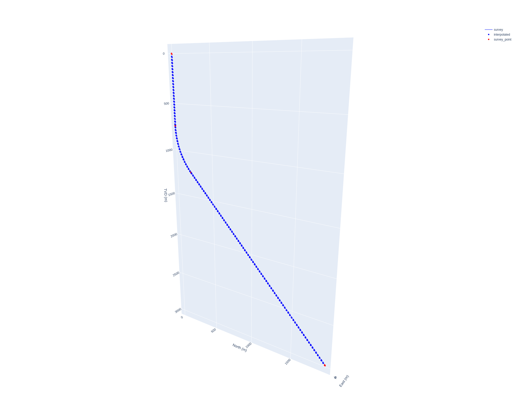 Plotting the trajectory from Example 3
The red points are the control points and the blue points are interpolated points - it looks how it was intended so let’s move on.
The paper describes some high dogleg sections toward the section TD of the well, but since the purpose of this post is to show how to use the welleng torque_drag module, we’ll simplify things and ignore this.
Create a Drilling BHA
The paper describes a simple drilling Bottom Hole Assembly (BHA) that we can create using welleng’s BHA class.
# initiate a BHA instance
bha = we.architecture.BHA(
    name='8 1/2" Drilling BHA', top=0, bottom=3718, method="bottom_up")

# add some Drill Collars
bha.add_section(
    od=(6.5 * ureg.inches).to('meters').m,
    id=(4 * ureg.inches).to('meters').m,
    length=(372 * ureg.ft).to('meters').m,
    unit_weight=(146.90 * ureg('lbs / ft').to('kg / meters')).m * 9.81,
    name='6 1/2" DC'
)

# add some HWDP
bha.add_section(
    od=(4.5 * ureg.inches).to('meters').m,
    tooljoint_od=(6.375 * ureg.inches).to('meters').m,
    id=(4 * ureg.inches).to('meters').m,
    length=(840 * ureg.ft).to('meters').m,
    unit_weight=(46.90 * ureg('lbs / ft').to('kg / meters')).m * 9.81,
    name='5" HWDP'
)

# add the drill pipe back to surface
bha.add_section(
    od=(5.0 * ureg.inches).to('meters').m,
    tooljoint_od=(6.625 * ureg.inches).to('meters').m,
    id=(3.625 * ureg.inches).to('meters').m,
    length=None,
    unit_weight=(20 * ureg('lbs / ft').to('kg / meters')).m * 9.81,
    name='5" DP'
)
The BHA is initiated using the bottom_up method, which means that we start
adding components at the bottom of the string first and work our way back up to surface. We give the string a name and give it a top and bottom depth in meters.
Create a Well Bore
Finally, we need to define the well bore that we’re running the BHA in, which normally consists of a casing followed by an open hole section. The first step is to initiate a WellBore instance.
# initiate a WellBore instance
wellbore = we.architecture.WellBore(
    name='8 1/2" Hole Section', top=0, bottom=3718, method='top_down'
)

# add the casing
wellbore.add_section(
    od=9+5/8, id=8.5,
    bottom=3688 * 0.7,
    unit_weight=(68 * ureg('lbs / ft').to('kg / meters')).m,
    coeff_friction_sliding=0.39,
    name='production 9 5/8" casing'
)

# add the open hole section below the casing to the section TD
wellbore.add_section(
    od=None, id=8.5, bottom=3718, unit_weight=None,
    coeff_friction_sliding=0.39, name='8 1/2" OH'
)
After initiating the WellBore, giving it a name, defining the top and bottom depths in meters and using the ‘top_down’ method for adding sections (starting at surface and adding sections below), a 9 5/8” casing was added from surface, with an 8 1/2” open hole section beneath.
Note: welleng’s units module utilizes the excellent pint library for unit conversions.
Torque and Drag
It’s time to calculate the torque and drag, which is done by initiating a TorqueDrag instance and providing the Survey, BHA and WellBore objects created above, plus a friendly name.
t_and_d = we.torque_drag.TorqueDrag(
    survey=survey_example_2, wellbore=wellbore, string=bha,
    fluid_density=9.8 / 8.33,
    wob=10_000, tob=(2_000 * 1.356), overpull=50_000,
    name='8 1/2" Hole Section'
)
Additionally, we need to provide the well bore fluid_density which is the density of the fluid in the well bore in Specific Gravity (SG) and optionally we can provide the Weight on Bit wob, Torque on Bottom/Bit tob and the overpull, all in Newtons.
For a visual QAQC of the results, the following convenience method can be used that generates a plotly figure:
>>> t_and_d.figure().show()
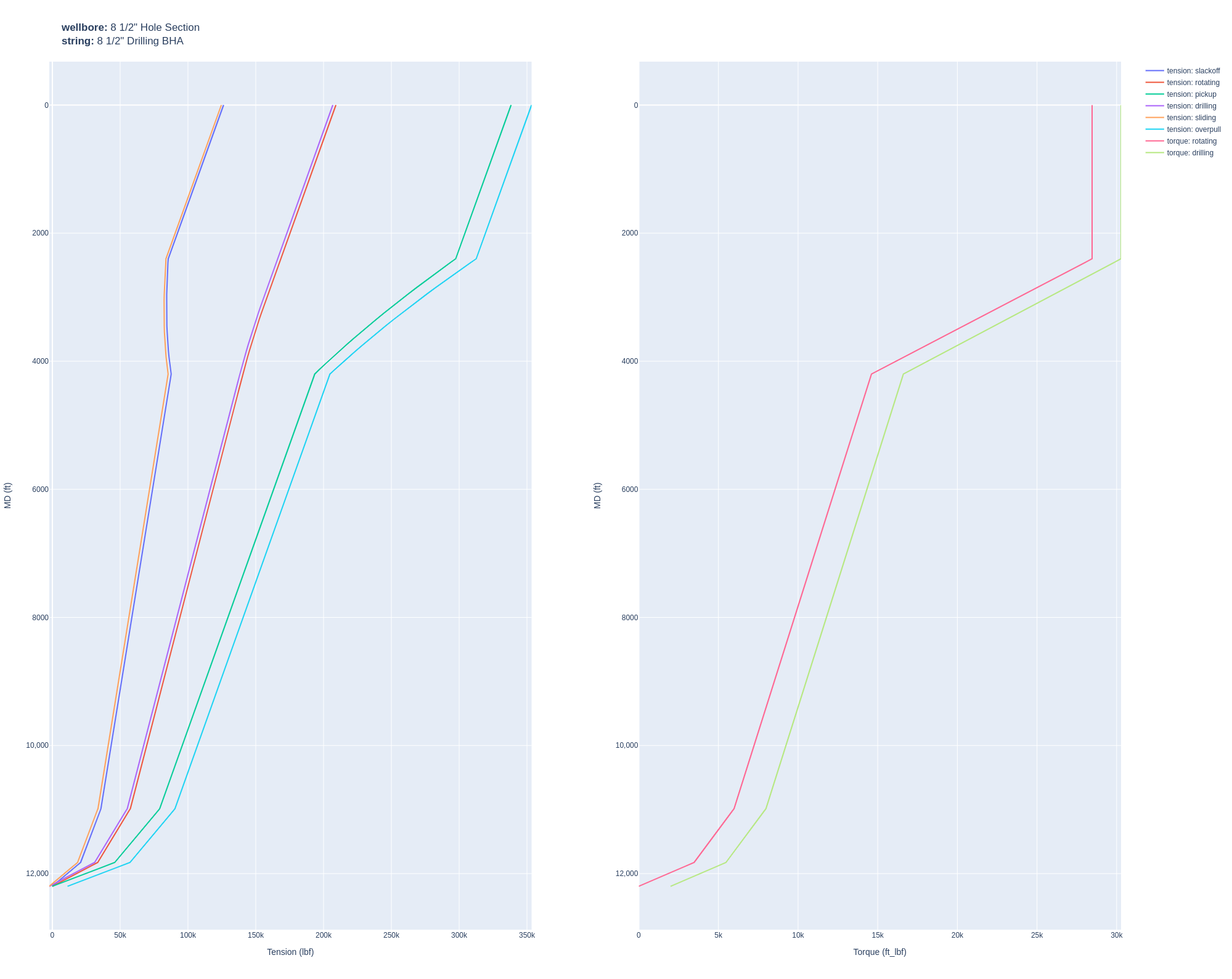 Torque and Drag plots for Example 3
Hook Load (Broomstick) Plot
Similarly, hookload data can be generated for a range of friction factors ff_range:
hookload = we.torque_drag.HookLoad(
    survey=survey_example_2, wellbore=wellbore, string=bha,
    fluid_density=11.6 / 8.33, step=30,
    name='8 1/2" Hole Section', ff_range=(0.1, 0.4, 0.1)
)
The ff_range denotes the from, to and step of the friction factor range.
For a quick visual QAQC of the results, the HookLoad class also has a convenience method for generating a plotly figure:
>>> hookload.figure().show()
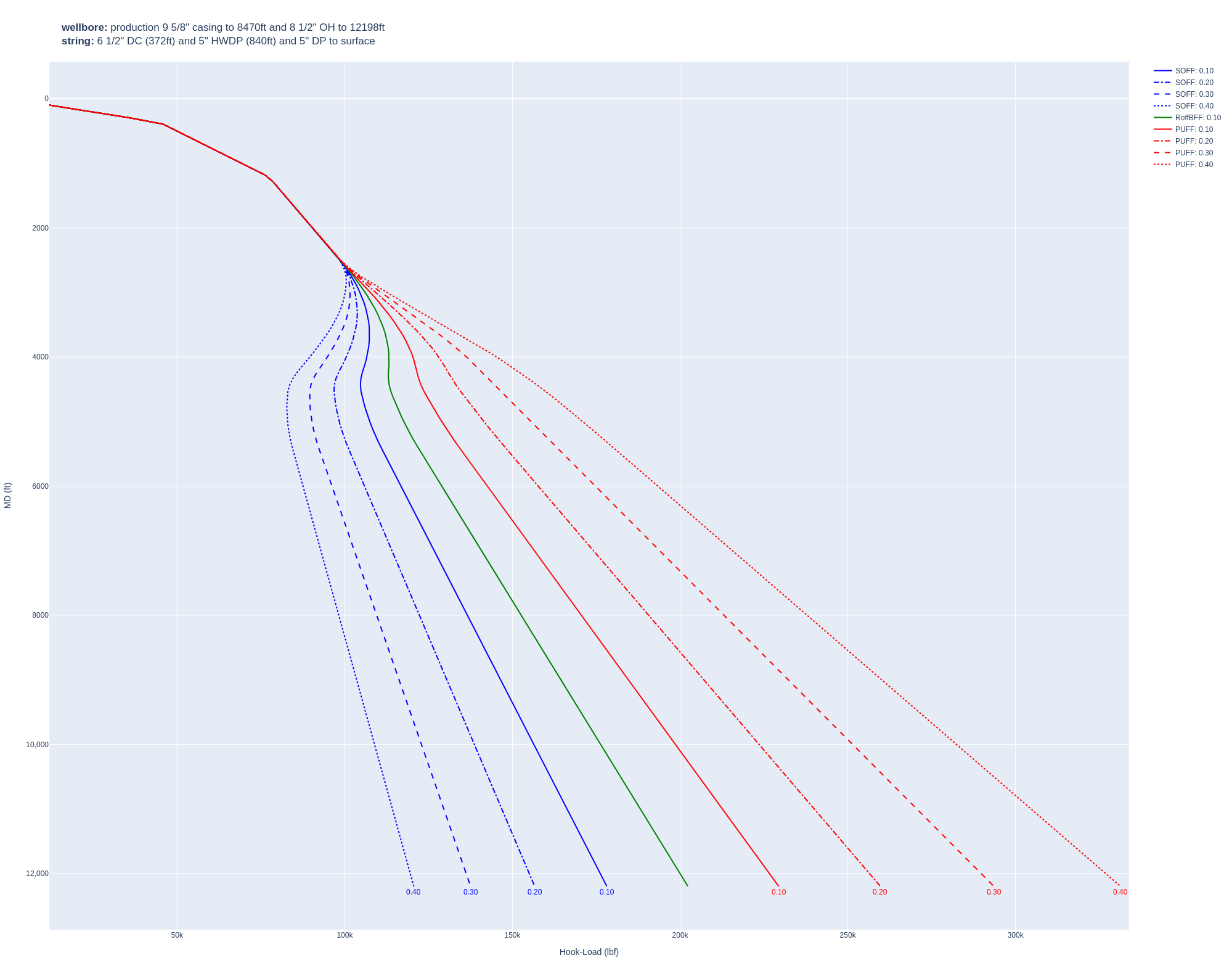 Hook Load or Broomstick plot for Example 3
Conclusion
The welleng library includes convenient methods for quickly generating Torque and Drag and Hook Load data for a given well trajectory and architecture. The calculations are simplistic and should therefore only be used as indicative, but for relative comparison of a range of trajectories they should be sufficient.
As usual, the Python script is available to use here. Please feel free to leave any comments or feedback.