Why Engineers should use Python
 Photo by Joseph Greve on Unsplash
There’s no doubting that spreadsheets like Microsoft’s ubiquitous Excel are a useful tool for QAQC of data, performing often complex maths functions and quick visualizations. It works great when the input data is nicely structured, ideally as Comma Separated Values (csv) or similar text format so that it can be loaded straight up.
But what happens when your data is not nicely tabulated and differs from row to row?
Dirty Data
In the real world, data is a mess and the bulk of the work is deciphering, cleaning and reformatting it into something that you can then work with. Spreadsheets are not the tool for this.
Here’s an example of some relatively messy data from which I needed to extract some parameters in order to troubleshoot some hardware issues. Below is a snip from a log file generated by PhoenixMiner, an application for mining Ethereum and other Proof of Work algorithms.
2021.08.19:07:44:05.125: eths Eth: Received: {"jsonrpc":"2.0","id":0,"result":["0xc4260ee73f727c0557f1c21e4651447a010a01d7ec43f0aa224bcd7ac4a44106","0x37f0818a24a483c5bd9c28e7b455358ccfe14a11e3504f5290946f9e3582775c","0x000000006df37f675ef6eadf5ab9a2072d44268d97df837e6748956e5c6c2116"]}
2021.08.19:07:44:05.964: main Eth speed: 175.484 MH/s, shares: 0/0/0, time: 0:00
2021.08.19:07:44:05.964: main GPUs: 1: 44.325 MH/s (0) 2: 43.529 MH/s (0) 3: 43.186 MH/s (0) 4: 44.444 MH/s (0)
2021.08.19:07:44:07.349: eths Eth: Received: {"jsonrpc":"2.0","id":0,"result":["0x8988682eda2b3f937d668c676bcebdfe2920ba26f53c888db3c0a5eceda95c7f","0x37f0818a24a483c5bd9c28e7b455358ccfe14a11e3504f5290946f9e3582775c","0x000000006df37f675ef6eadf5ab9a2072d44268d97df837e6748956e5c6c2116"]}
2021.08.19:07:44:07.349: eths Eth: New job #8988682e from eth-eu1.nanopool.org:9999; diff: 10000MH
2021.08.19:07:44:10.025: main GPU1: 67C 47% 126W, GPU2: 53C 46% 128W, GPU3: 54C 21% 109W, GPU4: 51C 20% 111W
GPUs power: 474.0 W; 370 kH/J
2021.08.19:07:44:10.926: eths Eth: Received: {"jsonrpc":"2.0","id":0,"result":["0x36bc7802b63cfae0d87f3df627ba6d70ac8e0349662f55270427a56ba6e8d4af","0x37f0818a24a483c5bd9c28e7b455358ccfe14a11e3504f5290946f9e3582775c","0x000000006df37f675ef6eadf5ab9a2072d44268d97df837e6748956e5c6c2116"]}
2021.08.19:07:44:10.927: eths Eth: New job #36bc7802 from eth-eu1.nanopool.org:9999; diff: 10000MH
2021.08.19:07:44:11.041: main Eth speed: 180.285 MH/s, shares: 0/0/0, time: 0:00
2021.08.19:07:44:11.041: main GPUs: 1: 45.357 MH/s (0) 2: 45.360 MH/s (0) 3: 44.080 MH/s (0) 4: 45.487 MH/s (0)
2021.08.19:07:44:13.444: eths Eth: Received: {"jsonrpc":"2.0","id":0,"result":["0x5ad73593ab0959c12aec1a3c1cac97d069d6db4a00a38388a8e914defe3afbbc","0x37f0818a24a483c5bd9c28e7b455358ccfe14a11e3504f5290946f9e3582775c","0x000000006df37f675ef6eadf5ab9a2072d44268d97df837e6748956e5c6c2116"]}
2021.08.19:07:44:13.444: eths Eth: New job #5ad73593 from eth-eu1.nanopool.org:9999; diff: 10000MH
2021.08.19:07:44:15.103: eths Eth: Send: {"id":5,"jsonrpc":"2.0","method":"eth_getWork","params":[]}
As you can see, this log data is not spreadsheet friendly as it differs from line to line. However, on closer inspection, there are some rows in the file that seem to repeat from which a template can be made and used to extract useful data. What I’m specifically interested in are the temperatures, fan speeds, power consumption and hash rate of the GPU cards in my four card mining machine.
Crack the Code
It helps having prior knowledge of how something works, and log files are no exception. Reviewing the data, it looks like each row begins with a date and time stamp. That will be useful as the x-axis of the charts I want to plot and it also provides a unique index for each row that could be useful later on.
Hash rate is usually measured in hashes per second or a multiple thereof, so numbers with MH/s units are references to hash rates. I know I have four GPUs, so where 1, 2, 3 and 4 are referenced (either alone or prefixed with GPU) is likely data associated with that specific GPU. The tag main GPUs: appears exclusively in the rows that indicate the hash rates - that can be used as a trigger for extracting that data!
Along with the GPU data I can see numbers with C, % and W suffixes which will undoubtedly refer to temperature (degrees C), fan speed (as a percentage of full speed) and power (in Watts) respectively. The tag main followed by a reference to the first GPU (in this case GPU1) appears exclusively in these rows with performance data - another trigger identified for extracting the desired data!
When writing code it’s good practice to make it as generic as possible so that it can be reused and is not specific for just your application. Along these lines, it’s reasonable that if someone wants to use our code then their miner may have more or less GPUs installed. It’d be nice if we could count them.
Looking at the log file when the PhoenixMiner application is initializing, reveals these lines:
2021.08.19:07:43:10.716: main Available GPUs for mining:
2021.08.19:07:43:10.716: main GPU1: Radeon RX Vega (pcie 3), OpenCL 2.0, 8 GB VRAM, 56 CUs
2021.08.19:07:43:10.716: main GPU2: Radeon RX Vega (pcie 6), OpenCL 2.0, 8 GB VRAM, 56 CUs
2021.08.19:07:43:10.716: main GPU3: Radeon RX Vega (pcie 10), OpenCL 2.0, 8 GB VRAM, 56 CUs
2021.08.19:07:43:10.716: main GPU4: Radeon RX Vega (pcie 13), OpenCL 2.0, 8 GB VRAM, 56 CUs
Here we can use the main Available GPUs for mining tag as a trigger to start counting the number of GPUs. It might also be possible to see how many GPUx tags there are, but knowing how the configuration file works for PhoenixMiner, some users may not be running all their GPUs and so the indexing might not be transparent.
Let’s start coding…
Importing data from the log file
Let’s write a function to import data from the log file, row by row via a generator (so not saving the data to memory unless we write some code to do so).
N_GPUS = 0

def import_data(filename):
    counting_gpus = False
    global N_GPUS
    with open(filename) as f:
        data = {}
        for row in f:
            row = row.strip("\n")

            if counting_gpus:
                if "GPU" in row:
                    N_GPUS += 1
                    continue
                else:
                    counting_gpus = False

            if "Available GPUs for mining" in row:
                counting_gpus = True
                continue

            if "main" in row:
                if "GPUs" in row:
                    data.update(get_gpu_hash_rates(row))
                else:
                    try:
                        data.update(get_gpu_data(row))
                    except (IndexError, NameError, TypeError, ValueError):
                        continue

    df = data_to_df(data)

    return df
We start off defining a global variable with the total number of GPUs (initialized to zero until we have reason to believe there are some GPUs installed in our machine) which will be referenced in a number of the functions we will write. Global variables are generally discouraged in Python, but here it’s convenient and we’ll capitalize the variable name to remind us it’s global.
The import_data() function takes a string parameter input which is the filename of the log file. From the snip of the log file above, we know at some point we’ll need to start counting rows to determine the number of GPUs, so we initialize a variable called counting_gpus to act as a flag. We also call the global N_GPUS variable described above.
Next, we open up the log file and start iterating through it one row at a time. We’ll initialize a dictionary called data to store the parameters we want from the log file. Since we’re importing from a text file, there’s a \n character at the end of each line which we remove.
If we encounter the Available GPUs for mining trigger then we activate the counting_gpus flag and if the GPU string is in the subsequent rows we increment our N_GPUS variable. If there’s no GPU tag then we stop counting and reset the counting_gpus flag.
As indicated above, there’s two more tags that we’re looking for in the rows, the simplest of which to spot is main GPUs. For the second tag, we’ll be lazy and just send every row to our function to extract the performance data: if it works properly then great, otherwise c’est la vie and we move to the next row - this is the purpose of teh try and except lines.
Since we want to plot the data we extract (or maybe even import it into a spreadsheet), we’ll convert the data dictionary to a pandas DataFrame instance - I generally try to avoid using pandas since it’s overkill for many tasks, but in this case it simplifies things quite a bit.
The import_data() function returns the DataFrame which we’ll subsequently pass to a plot function.
Hash Rates
Here’s the get_gpu_hash_rates() function for extracting the hash rates from a log file row for each GPU.
def get_gpu_hash_rates(row):
    time_stamp = get_time_stamp(row)
    gpus_data = row.split('GPUs: ')[1:][0]
    data = {
        time_stamp: {}
    }
    for n in range(N_GPUS):
        rate, unit = gpus_data.split(f"{n+1}:")[1].split(" ")[1:3]
        data[time_stamp][n + 1] = dict(
            rate = float(rate),
            unit = unit
        )
    if bool(data[time_stamp]):
        return data
    else:
        return
The first line calls a helper function that extracts the date and time stamp (remember that this is the start of every row in the log file) - we’ll look at that function in more detail below.
The next line is splitting the row at the GPUs tag and assigning the string to the right of the tag to the variable gpus_data. A dictionary is then created named data with the first key set as an empty dictionary with the key set to the time_stamp string variable.
The format of the hash data follows a template, where the GPU card and : suffix are followed by that card’s hash rate and hash rate unit (and a number in brackets, which we’ll not process for now but which refers to the number of successful shares achieved by that GPU). So in out code, for each GPU card we split the row at the reference to that GPU, take the right hand portion of that split string and then split that again on the space character “ “. We know that the first two words in this list of strings will be the hash rate and the hash rate unit respectively, so we assign these to variables and then create a dictionary entry for the current time stamp, with rate and unit keys respectively.
Once we’ve iterated through our list of GPUs then we return our new dictionary, but in case the dictionary is empty (perhaps we use a try) then we instead return a None to make it easier to process and clean up afterwards.
Date Time
Date and time strings can be a bit of a nuisance. The ones listed in this log file are almost in an ISO format, but not quite and therefore need to be fettled a little. Since the time stamps are listed on every row and will be used as the index and x-axis of our charts, it’s important to get them into a format that can be read as a time stamp.
First, here’s a quick helper function to extract the time data from a row.
def get_time_stamp(row):
    time_stamp = row.split(': ')[0]
    return time_stamp
Although the : character is used as a separator in the time stamp, the final colon has a space character suffix which you use to split the row, taking the left side of the split and returning this string as the time stamp.
Now we hae the time stamp string, we need to process it into an ISO format with this function:
def convert_to_datetime(time):
    time_new = list(time.replace(".", "-"))
    time_new[-4] = "."
    time_new[10] = " "
    time_new = "".join(time_new)
    return time_new
Here we take the time stamp string and replace the . characters with - characters and convert the string into a list of characters which we can then index. Unfortunately, this replaces the valid decimal place for the seconds in the time, so we need to convert this character back to a decimal point. Fortunately, this character always occurs 4 places from the end of the string, which we can now index after having converted our string to a list of characters.
The ISO format separates the date part of the string from the time part of the string with a space character. With these time stamps, the space separator is a colon character which is always at the 10th position in the string - so we can replace that colon with a space character.
All that’s left now is to convert our list of characters back into a string using the .join() operator and then return the reformated time stamp.
Performance Data
Next we want to extract the performance data for each GPU, namely the temperature, fan speed and power. This is slightly more difficult because the log data this time uses a prefix of GPU with the GPU numbers which we need to deal with.
Here’s the function for extracting the performance data from a row:
def get_gpu_data(row):
    time_stamp = get_time_stamp(row)
    gpus_data = row.split('main ')[1:][0]
    data = {
        time_stamp: {}
    }
    for n in range(N_GPUS):
        temp, fan, power = gpus_data.split(f"GPU{n+1}:")[1].split(" ")[1:4]
        temp, temp_unit = split_units(temp)
        fan = float(fan.strip("%"))
        power, _ = split_units(power)
        data[time_stamp][n + 1] = dict(
            temp = temp,
            temp_unit = temp_unit,
            fan = fan,
            power = power
        )
    if bool(data[time_stamp]):
        return data
    else:
        return
We start by extracting the time stamp with our previously described helper function. The GPU data is contained in the part of the row to the right of the tag main , so we extract that and assign it to the variable gpus_data.
Next, as for the hash rate data, we initiate our dictionary with a key (an empty dictionary) set to the time stamp. We then iterate through our GPUs to create our tags for splitting the row using a convenient f-string method. Each time we split at the GPUx: tag, we know that the first word is the temperature, the second word is the fan speed and the third word is the power - the data follows a set template. The unit for each parameter is the last character of the word, so we can split each word into the parameter and its unit and assign these to variables. We can create a helper function for this unit splitting:
import re

def split_units(string):
    value, unit = re.findall(r"[^\W\d_]+|\d+", string)
    value = float(value)
    return (value, unit)
We’re using re to make a template for the split, as we know the data is numeric and the unit is alpha.
Next, we can add keys and their values to out dictionary and return the dictionary, again checking that the dictionary is not empty.
Rinse, Wash, Repeat
The beauty of writing modular code is that once it’s working for one instance, it can then be used for every instance. By writing a function to conditionally process a row from a log file, we can then iterate through the log file and keep re-using the function, row by row.
This is precisely what our import_data() function is doing, pushing each row to the appropriate function for processing, receiving back a bit of dictionary which it then appends to a main dictionary - since our time stamps are unique then there’s no risk of overwriting entries in the main dictionary.
Reformat extracted data
Once the data of interest is extracted from the log file, it’s time to generate a table that we can use to create our charts. For simplicity, we’ll use the pandas library for this:
import pandas as pd
from copy import copy

def data_to_df(data):
    headers = list(get_headers(data))
    arr = []
    for time, gpus in data.items():
        temp = [None] * len(headers)
        for gpu, values in gpus.items():
            for k, v in values.items():
                temp[headers.index(k)] = v
            temp[headers.index('gpu')] = gpu
            temp[headers.index('time')] = convert_to_datetime(time)
            arr.append(copy(temp))

    df = pd.DataFrame(
        data=arr,
        columns=headers
    )

    df['time'] = pd.to_datetime(df['time'])

    return df
First step is to create a(n ordered) list of headers that we’ll use as the column headers in our pandas DataFrame instance. We’ll use a helper function for this that we send our dictionary of data to and receive back a list of all the data keys. This list is pre-populated with time and gpu as we know that these variables are in the data, but otherwise this function is written to have no pre-conceptions, so can accommodate future updates to the code where additional metrics might be extracted from the log data.
Note that copy is used when appending temp to arr - if you want to know why then read up on mutable versus immutable.
def get_headers(data):
    headers = set(['time', 'gpu'])
    for time, gpus in data.items():
        for _, values in gpus.items():
            for k in values.keys():
                headers.add(k)
    return headers
Now we have a list of headers, we can use this list to generate a table, since the length of the headers list defines the number of columns in the table and this list can be used ensure that the values in the dictionary are assigned to the correct columns.
Our table is initiated as an empty list and each row of the table is initiated as a list of None values with the same length as our headers list. The rationale for this is that missing data will default to None values in our table as it is constructed.
Perhaps now is a good time to see what our data dictionary looks like? One of the reasons I almost exclusively use an Integrated Development Environment (in my case Visual Studio Code) versus say Jupyter Notebooks is the ease of debugging and setting breakpoints in the code to delve into what’s happening into the background. So to see what the data dictionary looks like, I can set a breakpoint in the import_data() function and with the debug console:
>>> import pprint
>>> pprint.pprint(list(data.items())[:2])
[('2021.08.19:07:43:14.993',
  {1: {'fan': 14.0, 'power': 5.0, 'temp': 57.0, 'temp_unit': 'C'},
   2: {'fan': 13.0, 'power': 4.0, 'temp': 36.0, 'temp_unit': 'C'},
   3: {'fan': 21.0, 'power': 3.0, 'temp': 38.0, 'temp_unit': 'C'},
   4: {'fan': 20.0, 'power': 3.0, 'temp': 36.0, 'temp_unit': 'C'}}),
 ('2021.08.19:07:43:20.099',
  {1: {'rate': 0.0, 'unit': 'MH/s'},
   2: {'rate': 0.0, 'unit': 'MH/s'},
   3: {'rate': 0.0, 'unit': 'MH/s'},
   4: {'rate': 0.0, 'unit': 'MH/s'}})]
Here we import pprint and use it to print the first two entries of the data dictionary. Each entry in the dictionary has a unique time stamp as the key and there’s a dictionary within each entry. Each subitem has a key referenced to the GPU number and there’s either hash rate data or performance data for each GPU along with unit information.
So back to our data_to_df() function, for each time stamp, we iterate through each GPU and extract the data to the correct index of our temp row (using the header list to lookup the index). Once the temp row is constructed, we append it to our arr list and move to the next data entry, repeating until we’ve iterated through the entire data dictionary.
Once we constructed our table, it’s simple to convert it into a pandas DataFrame instance, but before we return the df, the time data is explicitly converted into datetime type so that it’s treated as a time series.
We now have a DataFrame and at this point we could export our table to a spreadsheet format and import it into e.g. Microsoft Excel. But anything that can be done in Excel can be done in Python…
Creating Charts
We set out to plot charts of mining data to see if it gave us some insight on the miner’s performance. So let’s make a function that takes our DataFrame and uses it to generate some charts.
A separate chart is required for each GPU, with time on the x-axis and the performance data on the y-axis. Fortunately, the performance data is all of the same order of magnitude, so no scaling of the data or multiple y-axis scales are required.
from plotly.subplots import make_subplots
import plotly.graph_objects as go

def plot(df):
    gpus = df['gpu'].unique()
    subplot_titles = [f"GPU{gpu}" for gpu in gpus]

    fig = make_subplots(
        rows=N_GPUS, cols=1,
        subplot_titles=subplot_titles
    )

    traces = {
        'temp': 'red',
        'power': 'green',
        'fan': 'blue',
        'rate': 'magenta'
    }

    for trace, color in traces.items():
        for i, gpu in enumerate(gpus):
            legendgroup = f"GPU{gpu}"
            temp = df.loc[(df['gpu'] == gpu) & (df[trace].notnull())]
            fig.add_trace(
                go.Scatter(
                    x=temp['time'],
                    y=temp[trace],
                    name=trace,
                    mode='lines',
                    line=dict(
                        color=color
                    ),
                    legendgroup=legendgroup,
                ),
                row=i + 1, col=1
            )

    fig.update_layout(
        height=N_GPUS * 300,
        legend_tracegroupgap=300 - 90,
        template='plotly_dark'
    )

    yaxis_range = [min(df['power'])-10, max(df['power'])+10]

    for i, gpu in enumerate(gpus):
        yaxis_label = "yaxis" if i == 0 else f"yaxis{i + 1}"
        fig.layout[yaxis_label]['range'] = yaxis_range

    return fig
We’re using make_subplots to generate a chart for each GPU, with a single column of charts. We define up front what traces we want to plot and the color associated to each, so that we can be consistent in every subplot.
Using the for loops, we slice up our df to create a view of each GPU’s data. For each view, we cycle through and extract the trace column, skipping any None or NaN values in the column. Once we’ve sliced our trace data, we add it to the appropriate subplot of our fig object, using out traces dictionary to assign the correct color. We also assign the legend to the appropriate GPU chart… currently plotly isn’t the best visualization tool for handling legends on subplots, but I’m sure they’re working on that.
Once the charts have been generated, the fig.layout is updated to set the height of the chart and position the legends in the correct location. A plotly_dark template is assigned to make it look pretty and a bit more hacker looking.
Finally, the y-axis ranges are set manually to be the same for each subplot.
Results
Time to test. The code below can be added to the Python script to import an explicit log file from a data folder in the same directory as the code is run from.
if __name__ == '__main__':
    import path

    PATH = os.path.dirname(os.path.realpath(__file__))

    filename = os.path.join(PATH, *("../data", "log20210819_074306.txt"))

    N_GPUS = 0

    df = import_data(filename)

    fig = plot(df)

    fig.show()
Note that the global N_GPUS variable needs to be set here.
Running this file results in the following plot.
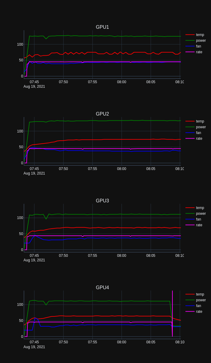 Charting PhoenixMiner performance data
Something weird is happening with GPU4 as the hash rate around 08:08 hrs falls off to zero before rocketing to the skies, with an associated drop in power, temp and fan speed. Clearly that warrants some further investigation.
Conclusion
Hopefully this post has provided some incentive to become less dependent on spreadsheets and instead use programming tools like Python to explore and visualize data. We’ve seen that with Python it’s possible to iterate through relatively messy data and extract relevant data based on repeating keywords or tags, all with free to use and often open source libraries.
As usual, the Python script is available to use here.