Density Downhole Changes in Static Fluids
This post will step through how to take a bunch of equations from a science paper (in this case Mathematical Field Model Predicts Downhole Density Changes in Static Drilling Fluids) and convert them into usable Python code.
Where to start
A good SPE paper will normally start with an abstract, then an introduction and then some theory before getting into the maths that leads to the final conclusion or formula. It’s always good to read the paper through and try and understand it, but invariably it’ll not make any sense whatsoever the first time round.
What’s clear from this paper is that we’re going to need to define some constants and a fluid with some reference properties. Since the determination of densities will be specific for the fluid that we define, a Pythonic way to do this will be to define a Fluid class and some class methods that will perform some calculations within the Fluid class.
Define the constants
We’ll first define some constants. This paper is written using API oilfield units - we’re just going to honor that for now and now worry about conversions, since this can be done simply later on. The following constants are defined in the paper and we’re going to make these globals which in Python are defined as variables with capitals:
# Define constants
A = [7.24032, -2.84383e-3, 2.75660e-5]
B = [8.63186, -3.31977e-3, 2.37170e-5]

# Gravitational constant
G = 0.052
When we define our fluid, we want to input as little information as possible. Based on experience, drilling fluids are simplistically made up from a base fluid (which is invariably a combination of water and/or (synthetic) oil), some weighting material (typically Barite) and a bunch of additives. For now we’ll ignore salts/brines and define our fluid as having a certain ratio of (fresh) water in the base fluid, using a specific weighting material and having a specific reference pressure, temperature and density (surface conditions).
We’ll start building a dictionary of weighting material properties - for now we’ll add this as a global but as this starts to grow it’d be better to store this as a separate file and import it, probably as a YAML or JSON file.
# Weighting Material Density in ppg
WEIGHTING_MATERIAL_DENSITY = {
    'barite': 35.,
    'spe_11118': 24.
}
The second entry in the dictionary above is back calculated from the example in the paper - practically, a drilling fluid will contain a range of solids that will include Low Gravity Solids, which effectively increase the relative volume of solids in a fluid for a given fluid density.
Define the class
Let’s start writing that class:
import math
from scipy.optimize import minimize
from numba import njit
import numpy as np

class Fluid:
    def __init__(
        self,
        fluid_density,
        reference_temp=32.,
        reference_pressure=0.,
        base_fluid_water_ratio=0.2,
        weighting_material='Barite'
    ):
        """
        Density profile calculated from SPE 11118 Mathematical Field Model
        Predicts Downhold Density Changes in Static Drilling Fluids by Roland
        R. Sorelle et al.

        This paper was written in oilfield units, so we'll convert inputs to
        ppg, ft, F and psi.

        Parameters
        ----------
        fluid_density: float
            The combined fluid density in ppg at reference conditions.
        reference_temp: float (default 32.0)
            The reference temperature in Fahrenheit
        reference_pressure: float (default 0.0)
            The reference pressure in psig.
        weighting_material: str
            The material being used to weight the drilling fluid (see the
            WEIGHTING_MATERIAL_DENSITY dictionary).
        """

        # check that the provided weighting material is in the dictionary
        assert weighting_material.lower() in WEIGHTING_MATERIAL_DENSITY.keys(), 'unknown weighting material'

        self.density_weighting_material = (
            WEIGHTING_MATERIAL_DENSITY.get(weighting_material.lower())
        )
        self.density_fluid_reference = fluid_density
        self.temp_reference = reference_temp
        self.base_fluid_water_ratio = base_fluid_water_ratio
        self.pressure_reference = reference_pressure
That’s the basic Fluid class initiated. We now need to determine the densities of our base fluids at the reference conditions - when we quote a density of a fluid it’s invariably at standard conditions, so we need to know what they are at the temperature and pressure conditions when the fluids were tested.
Here’s the internal method for calculating these based on equations 1 and 2 from the paper (we hint that the method is for internal use with the single underscore prefix):
def _get_density_base_fluids(self):
    """
    Equation 1 and 2
    """
    def func(temperature, pressure, c):
        density = c[0] + c[1] * temperature + c[2] * pressure

        return density

    self.density_oil_reference = func(
        self.temp_reference, self.pressure_reference, A
    )
    self.density_water_reference = func(
        self.temp_reference, self.pressure_reference, B
    )
We’ve written an internal function here since the form of the equations for calculating density for water and oil is the same, just with difference constants. A and B are the globals we defined earlier.
Now we have the densities for our base fluid, we need to calculate some relative volumes for our water, (synthetic) oil and our solids. We’ll write another internal method for this:
def _get_volumes_reference(self):
    # calculate our base fluid average density
    self.base_fluid_density_reference = (
        self.base_fluid_water_ratio * self.density_water_reference
        + (1 - self.base_fluid_water_ratio) * self.density_oil_reference
    )

    # calculate how much weighting material is required to bulk
    # up our base fluid to the desired drilling fluid density
    volume_weighting_material = (
        self.density_fluid_reference
        - self.base_fluid_density_reference
    ) / self.density_weighting_material

    volume_total = 1 + volume_weighting_material

    # calculate our unit volume ratios
    self.volume_water_reference_relative = (
        self.base_fluid_water_ratio / volume_total
    )
    self.volume_oil_reference_relative = (
        (1 - self.base_fluid_water_ratio) / volume_total
    )
    self.volume_weighting_material_relative = (
        volume_weighting_material / volume_total
    )
Now that we have some internal methods for calculating these fluid properties, we need to call them in our class’ __init__() function by adding the following two lines:
self._get_density_base_fluids()
self._get_volumes_reference()
That’s our class initiated!
Define the class method
We’ve define a fluid, but now need to add a method for calculating the fluid’s density profile versus True Vertical Depth (TVD) for a given temperature profile and applied pressure. If we take a look at the SPE paper, we can jump to the end of the mathematical section to equation 32 - this is the equation that we need to solve to get the average density for a given depth and temperature relative to the reference properties.
Looking at equation 32, there’s some coefficients that we need to calculate, \(\alpha_1, \alpha_2, \beta_1, \beta_2\) in equations 28 - 31, so let’s write a static method to determine these:
@staticmethod
def _get_constants(
    density_average, pressure_applied, temperature_top,
    fluid_thermal_gradient, A0, A1, A2, B0, B1, B2
):
    alpha_1 = (
        A0 + A1 * temperature_top + A2 * pressure_applied
    )
    alpha_2 = (
        A1 * fluid_thermal_gradient + G * A2 * density_average
    )
    beta_1 = (
        B0 + B1 * temperature_top + B2 * pressure_applied
    )
    beta_2 = (
        B1 * fluid_thermal_gradient + G * B2 * density_average
    )

    return (alpha_1, alpha_2, beta_1, beta_2)
There’s a reason why this is written as a static method and why the A and B globals are broken out, which we’ll discuss later.
Things get a bit more interesting now, because the main equation has \(\rho_a\) on both sides (and also in the _get_constants() method above) and although it’s alluded to in the paper that an iterative method is required to solve the equation, there’s no example to demonstrate such a method.
We’re going to use the scipy optimize.minimize method to solve this equation, because it’s fast and relatively simple to use. Let’s first code up our internal static method:
@staticmethod
def _func(
    density_average, density_top, volume_water_relative,
    volume_oil_relative, depth, alpha_1, alpha_2, beta_1, beta_2
):
    # if the depth is zero we return our reference density and
    # avoid a divide by zero error
    if depth == 0:
        return density_top
    func = (
        (
            density_top * depth
            - (
                volume_oil_relative * alpha_1 * density_average
                / alpha_2
            )
            * math.log(
                (alpha_1 + alpha_2 * depth) / alpha_1
            )
        ) / (depth * (1 - volume_water_relative - volume_oil_relative))
        - (
            volume_water_relative * beta_1 * density_average / beta_2
            * math.log(
                (beta_1 + beta_2 * depth) / beta_1
            )
        ) / (depth * (1 - volume_water_relative - volume_oil_relative))
    )
    return func
Both of these internal static methods must be called for each iteration, where in each iteration we make an estimate of the \(\rho_a\) property. If we’ve estimated the \(\rho_a\) correctly, then the _func() method will return the same value as the estimated \(\rho_a\) value.
The minimize method uses a clever iterative method to minimize a scalar function, so we need to write an internal method that will return an error value and have the minimize method minimize this error.
def _get_density(
    self, density_average, density_top, temperature_top,
    volume_water_relative, volume_oil_relative, pressure_applied, depth,
    fluid_thermal_gradient
):
    # the minimize method makes a list of the x0 (density_average)
    # so we need to pick the first (and only) item from this list
    density_average = density_average[0]

    # calculate out coefficients
    alpha_1, alpha_2, beta_1, beta_2 = self._get_coefficients(
        density_average, pressure_applied, temperature_top,
        fluid_thermal_gradient, A[0], A[1], A[2], B[0], B[1], B[2]
    )

    # calculate our density_average
    func = self._func(
        density_average, density_top, volume_water_relative,
        volume_oil_relative, depth, alpha_1, alpha_2, beta_1, beta_2
    )

    # return the error (difference between estimate and calculated
    # density_average)
    return abs(density_average - func)
It’s time to write our method for calculating the density profile:
def get_density_profile(
    self,
    depth,
    temperature,
    pressure_applied=0.,
    density_bounds=(6., 25.)
):
    """
    Function that returns a density profile of the fluid, adjusted for
    temperature and compressibility and assuming that the fluid's reference
    parameters are the surface parameters.

    Parameters
    ----------
    depth: float or list or (n) array of floats
        The vertical depth of interest relative to surface in feet.
    temperature: float or list or (n) array of floats
        The temperature corresponding to the vertical depth of interest in
        Fahrenheit.
    pressure_applied: float (default=0.)
        Additional pressure applied to the fluid in psi.
    density_bounds: (2) tuple of floats (default=(6., 25.))
        Density bounds to constrain the optimization algorithm in ppg.
    """

    # Convert to (n) array to manage single float or list/array
    # so that either single values or lists of depths can be handled
    depth = np.array([depth]).reshape(-1)

    # We need to hush up divide by zero warnings and replace NaN
    # values with zeros - the function is written with thermal
    # gradient as the input
    with np.errstate(invalid='ignore'):
        temperature_thermal_gradient = np.nan_to_num((
            temperature - self.temp_reference
        ) / depth
        )

    # our minimize function - it iterates through each depth and
    # temperature tuple
    density_profile = [
        minimize(
            fun=self._get_density,
            x0=self.density_fluid_reference,
            args=(
                self.density_fluid_reference,
                self.temp_reference,
                self.volume_water_reference_relative,
                self.volume_oil_reference_relative,
                pressure_applied,
                d,
                t,
            ),
            method='SLSQP',
            bounds=[density_bounds]
        ).x
        for d, t in zip(depth, temperature_thermal_gradient)
    ]

    # process the results to a nice flat list
    return np.vstack(density_profile).reshape(-1).tolist()
And we’re done!
Example
What’s nice about this SPE paper is that it provides an example that can be used to check if the functions have been coded correctly. So let’s recreate the worked example and see if we get the same result.
We’ll wrap this example in a main() function:
def main():
    """
    An example of initiating a Fluid class and generating a density profile
    for the fluid for a range of depths and temperatures.
    """
    # Define the fluid
    fluid = Fluid(
        fluid_density=10.,  # ppg
        reference_temp=120.,  # Fahrenheit,
        weighting_material='SPE_11118',
        base_fluid_water_ratio=0.103,
    )
The above code will create a Fluid instance with out fluid properties. However, the theoretical properties of this fluid do not quite match the values in the provided example. No problem… we’ll just modify them to exactly match the properties in the example:
fluid.volume_water_reference_relative = 0.09
fluid.volume_oil_reference_relative = 0.78
fluid.volume_weighting_material_relative = 0.11
We could just use the get_density_profile() method with the total depth and associated temperature, but instead we’ll calculate the values for every 10 feet.
# generate arrays of depths and temperatures
depth = np.linspace(0, 10_000, 1001)
temperature = np.linspace(120, 250, 1001)

# use out method to calculate the density profile
density_profile = fluid.get_density_profile(
    depth=depth,
    temperature=temperature
)
To check our result against the paper’s example, let’s call the last result:
>>> density_profile[-1]
9.852742609844203
This compares with the answer in the paper of \(\rho_a = 9.85\ lb/gal\)
Result!
Results
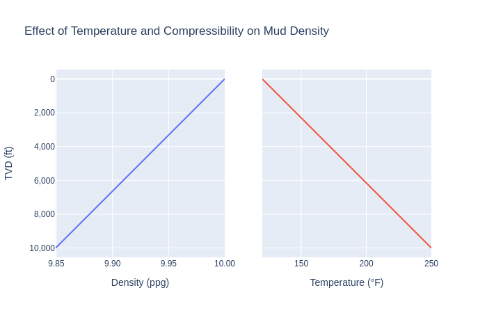
Let’s quickly write some code to visualize the results:
# load dependencies for plotting results
import plotly.graph_objects as go
from plotly.subplots import make_subplots

# construct plots
fig = make_subplots(rows=1, cols=2, shared_yaxes=True)

# add the density data
fig.add_trace(go.Scatter(
    x=density_profile,
    y=depth,
    mode='lines',
    name='Density (ppg)',

), row=1, col=1)

# add the temperature data
fig.add_trace(go.Scatter(
    x=temperature,
    y=depth,
    mode='lines',
    name='Temperature (F)'
), row=1, col=2)

# add titles and flip the y-axis
fig.update_layout(
    title="Effect of Temperature and Compressibility on Mud Density",
    yaxis=dict(
        autorange='reversed',
        title="TVD (ft)",
        tickformat=",.0f"
    ),
    showlegend=False
)

# upate x-axes titles and format the numbers
fig.update_xaxes(
    title_text="Density (ppg)",
    tickformat=".2f",
    row=1, col=1
)

fig.update_xaxes(
    title_text="Temperature (\xb0F)",
    tickformat=".0f",
    row=1, col=2
)

fig.show()
The result is… a bit boring. Since the temperature profile is assumed to be linear then the density results are also linear. What is interesting is that large temperature gradients result in a decrease in static mud gradient with depth.
Optimization
Back to why we wrote the code this way… since we’re iterating, it’s possible that our functions will be used quite heavily (although the minimize method is very efficient). Writing the functions this way enables us to use numba to speed them up with the addition of a simple decorator. Have a go at implementing this else feel free to download the code which is a module of the welleng Python library.